
About This Manual
Decompose documentation introduces the product, its concepts, and how to use it effectively. It is meant to orient new users and provide a quick path to the key workflows and references. Reading this manual helps you understand what the tool does and where to find specific guidance.
Introduction
Decompose is a collection of independent, specialized modules for modernizing legacy applications. These modules include Tracer, Insights, Decomposition, DB Cutting, and Code and Migration Generators.
There is also a utility tool called "Talk to Database" that uses AI to query databases for business insights. This capability highlights how the platform provides in-depth analysis of source code and database structures, enabling organizations to break down complex, monolithic systems into manageable components.
Users of Decompose must manually decide which data to migrate to the new microservice database. The platform automatically generates an initial design for the new database and provides reports to jump-start the ETL migration process.
Decompose is part of the Phaidon Modernization Platform. It extracts smaller databases from large legacy databases. These smaller databases are intended for use with microservices.
Decompose encourages users to think in terms of Domain-Driven Design. Martin Fowler provides a useful introduction to Bounded Contexts, a key concept within this methodology.
Installation
For installation instructions, see Installation Steps.
Basic concepts
This page introduces the core ideas behind Decompose and the terminology used throughout the product. It gives you the background needed to interpret the UI, workflows, and reports correctly. Read this page first if you are new to decomposition or want a shared vocabulary before moving into feature-specific guides.
Decompose
Most legacy applications and databases are monolithic and lack a clear separation of domains/contexts. When modernizing applications, we aim to decompose such monolith applications and databases following a domain-driven design approach by separating the data into contexts.
The Decompose Web UI is the central element of the Decompose application. Here the user can carve out new databases out of the existing legacy database by analyzing the data that each bounded context accesses. The page also provides tools to resolve conflicts between bounded contexts.
The user of Decompose has to manually decide what data is migrated to the new microservice database. Decompose will on the fly generate a first design for the new database, as well as provide reports to jump-start the ETL migration process. Details on the usage of Decompose can be found in the sub-sections of this documentation.
What is Decompose?
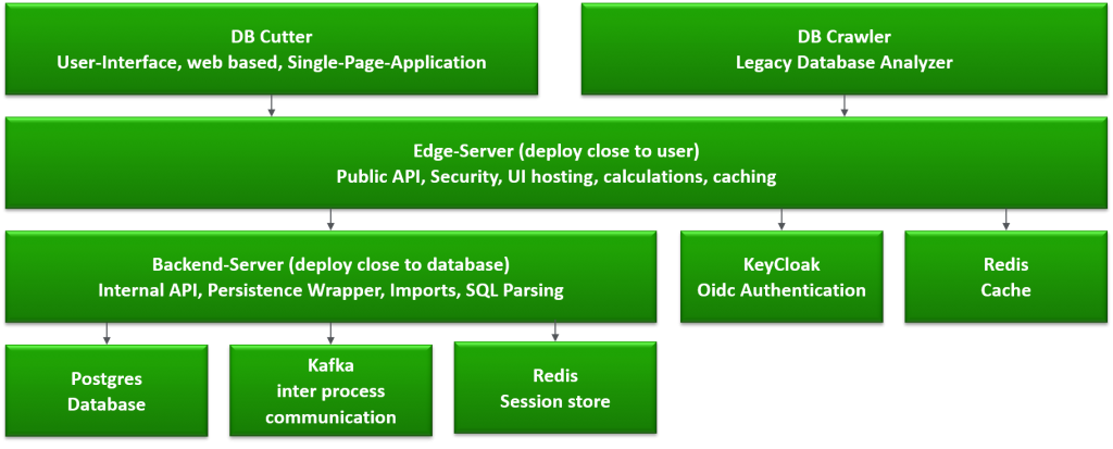
The Decompose consists of three main components:
-
Decompose Web UI
-
The DB Crawler
-
The backend with its database
The components are built as an n-tier architecture. The communication with the Phaidon stack, that is the Monolith Cutter, is done by using Apache Kafka as event-driven backplane. The figure below shows the relation between the user and the databases.
What is Decomposition?
When working on large legacy applications, you usually do not want to modernize that with a big bang release. Instead, you could want to modernize iteratively, moving parts of the old application to a new architecture and infrastructure.
The end goal is to iteratively migrate a monolithic application to a cloud native technology stack. For this purpose, the user chooses tables (or application endpoints) that belong together and creates Microservices from that, including source code and data.
-
You can create Taxonomies which means you tag a set of modules with a name
-
You can automatically tag modules that belong together to a sub-application
-
You can automatically tag modules that are accessing shared data
-
You can visually edit taxonomies
-
You can define sub-applications within your large legacy application. In Domain Driven Design, these would be called domains, or Bounded Contexts
-
You can ask the Decompose to automatically split your application into domains
What is a Bounded Context?
For the Decompose, it is essential to divide the the legacy application into a set of bounded contexts. Each bounded context can become a microservice, consisting of its own database.
Each bounded context contains multiple modules and may be shared between contexts.
A module is a class or code file of an arbitrary legacy language.
Each module can contain SQL queries to the legacy database. The Decompose investigates the queries and thus knows the relation between contexts, modules and data in tables/columns.
Environment setup
This page explains how to set up Decompose locally by using Docker. It covers the installation flow, the containers included in the standard deployment, and the main configuration values you may need to review. Use it as your baseline reference when preparing a local or project-specific environment.
Installation steps
Follow these steps in order to install the product and bring up the local services successfully. The sequence covers licensing, Docker prerequisites, registry access, and the initial startup flow. Review the notes in each step carefully because later features depend on a complete and healthy environment.
Step 1:
Obtain a valid Decompose license by reaching out to amiproductsupport@deloitte.com.
Step 2:
Install Docker for your respective operating system:
Step 3:
Open a command prompt and log into the GitLab container registry:
Info
This login step only needs to be executed once as your login credentials will be stored on your system.
Step 4:
To download and start the Decompose Docker containers, save the docker-compose.yaml file that was delivered in the Decompose release email to your local file system.
Step 5:
Place the license file innowake.lic (see step 1) into the same directory as the docker-compose.yaml.
Step 6:
Execute the following command in the same directory where the docker-compose.yaml resides:
For large customer projects, the default settings for Java heap sizes need to be adjusted.
The memory settings for db-cutter-service have to be adapted by adding an environment entry in the docker-compose.yaml, for example:
Docker Desktop also requires sufficient memory allocation.
Step 7:
Once the docker-compose command has finished, the Decompose can be accessed via your browser: http://localhost:5001/
The default user credentials are username "TruNorth Decompose" and password "password".
Docker containers
The standard Docker Compose package starts several containers that together provide the UI, backend services, identity management, storage, and messaging components. Understanding the role of each container helps you troubleshoot startup issues and size the environment appropriately. The following table summarizes the containers included in the default setup.
The following containers are pulled via the docker-compose.yaml:
| Container | Description |
|---|---|
| db-cutter-service | The core of the Unified Cutter. This spring boot application contains all the logic for importing data, processing data and providing data (REST API). |
| db-cutter-ui | The web server hosting the Blazor web UI of the Unified Cutter (interface to the end user). |
| keycloak | The service used for authentication and IAM (Identity and Access Management). This involves the login to the Unified Cutter, maintaining group privileges etc. |
| pgadmin | The UI for accessing the postgres database (only required for administrative purposes) |
| postgres | The relational database used to store the uploaded data (modules, queries, bounded contexts etc), project information and generated data which is produced by the Unified Cutter. |
| postgres-keycloak | The database used by the keycloak container to store IAM data. |
| redis | Needed by the db-cutter-service. It is used for storing temporary update data which can by fetched by clients (like progress updates for an import task). |
| Kafka | Apache Kafka is an open-source distributed event streaming platform. Used for event sharing, client and project CRUD events and logics will be managed by separate service, UI services will raise events to get request payloads and send back the response via Kafka topics. |
| MinIO | MinIO is a high-performance, S3 compatible object store. It is used for storing traced application logs. |
| Zookeeper | ZooKeeper is a centralized service for maintaining configuration information, naming, providing distributed synchronization, and providing group services. It is used for Kafka management. |
The list of backend server variables:
| Environment Variables | Definition/Description | Default Value | Format |
|---|---|---|---|
| DECOMPOSE_SERVER_PORT | Server port configuration with default value | 8080 | String |
| POSTGRES_URL | Database URL with default value | jdbc:postgresql://postgres:5432/dbcutter | String |
| POSTGRES_USER | Database username with default value | root | String |
| POSTGRES_PASSWORD | Database password with default value | Worx2000 | String |
| KAFKA_BOOTSTRAP_SERVERS | Kafka bootstrap servers with default value | kafka:29092 | String |
| USE_REDIS_AS_CACHE | Use Redis as cache with default value | true | String |
| REDIS_HOST | Redis host with default value | redis | String |
| REDIS_PORT | Redis port with default value | 6379 | String |
Types of roles
Decompose uses role-based access to separate administration, editing, and read-only activities. Knowing these roles helps you assign permissions that match each team member's responsibilities without granting unnecessary access. The table below summarizes the default role definitions.
| Role Name | Description |
|---|---|
| Manager | The Manager role has full access to the projects he was granted access to, can create new projects, can import data, can do manual edits, and add or remove viewers and/or editors to clients and projects they have access to. |
| Editor | The Editor role has access to the clients and projects they have access to, manual editing capabilities, and can import data. |
| Viewer | The Viewer role has read-only access to the clients and projects assigned to them and can view and export reports. |
Types of cache
There are two types of caches, a redis cache and an in-memory cache. The redis cache is the default and requires the redis container to get started. Both types of cache are used by the Decompose Service and Decompose UI. The in-memory cache was only added as a fallback strategy for situations in which the client does not want to use redis as a cache.
For the Decompose Server, we have a property called redis.use-redis-as-cache in our application.yaml file. To change the value, you can either edit the file inside the jar or start the Decompose Service with the following arguments:
-Dspring-boot.run.arguments="-redis.use-redis-as-cache=false".
We have an EnvironmentVariable.cs to change the cache behavior for the Decompose Service.
For the Decompose Client, we have a property called UseRedisAsCachein our appsettings.json file. To change the value you can either edit the file or set the environment variable Redis:UseRedisAsCache=false.
Environment variable
Frontend behavior is controlled through environment variables that define service endpoints, authentication settings, caching, and optional AI integrations. Review these values when you deploy the UI in a new environment or need to change defaults for an existing installation. The following table lists the available frontend variables and their purpose.
Below are the list of frontend variables:
| Environment Variables | Definition | Default Value | Format |
|---|---|---|---|
| DB_CUTTER_BACKEND_URL | It stores the URL where the UI-Server can find the backend service | http://db-cutter-service:5080/ | String |
| DB_CUTTER_APP_BASE_PATH | The base path of the application | / | String |
| REDIS_HOST | The host name of the redis server | redis | String |
| REDIS_PORT | The port of the redis server | 6379 | String |
| DB_CUTTER_USE_REDIS_AS_CACHE | True to enable redis as cache – otherwise in-memory cache is used | TRUE | String |
| DB_CUTTER_AUTHORITY | The oauth authority server from UI perspective | http://localhost:28080/realms/Phaidon-realm | String |
| DB_CUTTER_AUTHORITY_INTERNAL | The oauth authority server from server perspective | http://keycloak:8080/realms/Phaidon-realm | String |
| DB_CUTTER_RESPONSE_TYPE | The oauth response type, for example. “code” | code | String |
| DB_CUTTER_CLIENT_ID | The client id for keycloak, for example. “db-cutter” | db-cutter | String |
| DB_CUTTER_REDIRECT_URL | The redirect URL, where Keycloak sends an authenticated user | http://localhost:5001/ | String |
| DB_CUTTER_AUDIENCE | The Keycloak audience, for example, account | account | String |
| DB_CUTTER_ISSUER_ADDRESS | The Keycloak issuer address | http://localhost:28080/realms/Phaidon-realm/protocol/openid-connect/auth | String |
| DB_CUTTER_CONNECTIONSTRING | The connection string to the postgres database | Host=postgres;Database=dbcutter;Username=root;Password=Worx2000 | String |
| GEN_AI_AZURE_URI | The URI of the GPT instance | https://iw-dev-ai.openai.azure.com/ | String |
| GEN_AI_AZURE_KEY_CREDENTIAL | The ApiKey for GPT | 0004abba388e400492a1c65429d9c42b | String |
| GEN_AI_DEPLOYMENT_NAME | The deployment name of the GPT model, for example, gpt-4-32k. | "gpt-35-turbo" or "gpt-4-32k" or "gpt-4o" | String |
| GEN_AI_INFERENCE_TEMPERATURE | The inference temperature for GPT | 0.7 | String |
| GEN_AI_MAX_TOKENS | The maximum number of tokens returned by GPT | GPT3.5: 2k, for GPT4-32k: 10k, for GPT4o: 4k | String |
| GEN_AI_IS_GEN_AI_ENABLED | True to enable GenAI, else the Generator section in the UI is not shown. | TRUE | String |
| GEN_AI_TYPE | The type of GenAI that is used to generate content: “default” or “LlmService” | default or LlmService | String |
| LLM_SERVICE_SERVICE_ADDRESS | The URL of the LlmService container | "http://llmservice:8000" or "https://appmodil.deloitte.com/genai/staging/llm-service" | String |
| LLM_SERVICE_PLUGIN | The llm service plugin, for example. “azure gpt 3.5” or “azure gpt 4”. Must match a plugin that is configured in the LlmService container | "azure gpt 3.5" or "azure gpt 4" or "azure gpt omni" | String |
| LLM_SERVICE_INFERENCE_TEMPERATURE | The llm service inference temperature | 0.7 | String |
| LLM_SERVICE_MAX_TOKENS | The maximum number of tokens returned by the LlmService | for GPT3.5: 2k, for GPT4-32k: 10k, for GPT4o: 4k | String |
| DB_CUTTER_MIGRATE_DB_ON_STARTUP | Indicates whether this webserver will migrate the database schema to the current version on startup (true/false) | TRUE | String |
| DB_CUTTER_MIGRATE_DB_USER | The name of the database user that will become the owner of all migrated tables, that is, replaces ${flyway:user} | root | String |
| GEN_AI_DEPLOYMENT_NAME_EMBEDDING | The deployment name of the GPT model for embeddings, for example, gpt-4-32k | text-embedding-ada-002 | String |
| GEN_AI_EMBEDDING_MODEL | The embedding model to be used | text-embedding-ada-002 | String |
| QDRANT_HOST | qdrant | String | |
| QDRANT_PORT | 6334 | String | |
| QDRANT_SCORE_THRESHOLD | 0.5 | String | |
| IS_SEMANTIC_SEARCH_ENABLED | TRUE | String | |
| QDRANT_VECTOR_SIZE | 1536 | String | |
| QDRANT_RESULT_LIMIT | 1000 | String | |
| GEN_AI_STORE_TOKEN_USAGE | True to log all prompts for GenAi and used tokens in the database | FALSE | String |
| KAFKA_BOOTSTRAP_SERVER | The KAFKA_BOOTSTRAP_SERVER | kafka:29092 | String |
| KAFKA_CONSUMER_GROUP_ID | The KAFKA_CONSUMER_GROUP_ID | integration-group | String |
| INNOWAKE_SSL_DISABLE | To disable the SSL certificate check, set this variable to true | FALSE | String |
DB Crawler
The DB Crawler extracts structural metadata from a legacy database so that Decompose can analyze schemas, tables, and relationships. It is typically one of the first tools you use when preparing a project because many downstream features depend on imported schema information. Use this page when you need to generate the schema artifact or troubleshoot crawler-specific execution behavior.
Info
The db-crawler and database driver jars as well as access to the database are the prerequisites for DB Crawling.
For cutting a database and selecting a suitable target database, the user must first extract the schema file of the database to import it into the Decompose UI. Then the database can be further analyzed. This can be done using the DB Crawler.
For getting the db-crawler jar, please refer to Schema Upload.
For a first time login, the user might not have the schema file. To get the schema file download the crawler jar.
To extract the database schema json file, the user can run the following command:
java -Xmx8g -cp "db-crawler-<version>.jar:mssql-jdbc-9.4.0.jre8.jar" innowake.innovationlab.dbcrawler.Main -c "jdbc:sqlserver://localhost;databaseName=<database name> " -u <user name> -p <password> -f <filename>.json
The database driver jar must be compatible with the database version.
Allowing next on exhausted result set
The IBM Data Server Driver for JDBC and SQLJ automatically closes the cursor when all rows have been retrieved from a ResultSet. When ResultSet.next is executed after the cursor is closed, an SQLException is thrown. This behavior differs from the DB2 JDBC Type 2 drive, where the cursor is not automatically closed when all rows from a ResultSet have been retrieved. To avoid this, the user must pass the -DallowNextOnExhaustedResultSet=1 flag when executing the crawl command.
-DallowNextOnExhaustedResultSet=1 java -Xmx8g -cp "db-crawler-<version>.jar:mssql-jdbc-9.4.0.jre8.jar" innowake.innovationlab.dbcrawler.Main -c "jdbc:sqlserver://localhost;databaseName=<database name> " -u <user name> -p <password> -f <filename>.json DallowNextOnExhaustedResultSet=1
- IBM Support. More Support for: Db2 for Linux, UNIX and Windows. Software version: 9.7, 0.5, 91. Operating system(s): AIX; Linux, Solaris, Windows. Document number: 416563. Modified Date: 16 June 2018.
Getting started
After Decompose has been set up within your environment, you are ready to get started with the Decompose UI. This page walks through the first actions that help you enter the application, create a working project, and prepare your data for analysis. You may also access the playground environment to test out the available features in Decompose here.
Log in
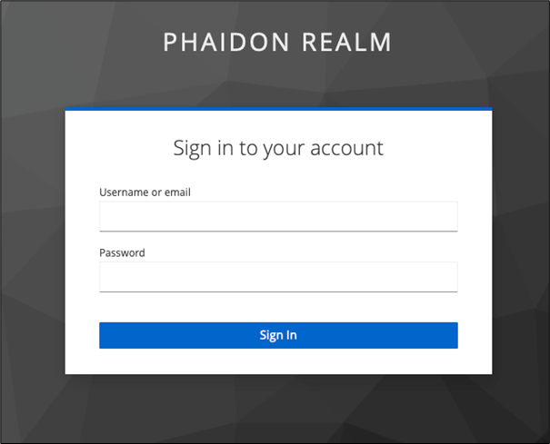
When accessing the UI, you will first be presented with a sign-in page displaying your environment's name. In the example below, "Phaidon Realm" represents the environment name. Enter your username or email and password in the provided fields.
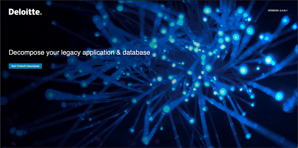
To begin, click Start Decompose to proceed to the Clients and Projects page.
Clients and projects
Setting up a client and a project provides the essential structure for your modernization efforts when you begin using Decompose. Creating a client allows you to keep data and activities for each organization or business unit logically separated. This supports security, easy management, and clean access control. Organizing work into projects beneath each client helps allocate resources efficiently, enables auditability and compliance tracking, and allows your teams to reuse processes as you scale your modernization initiatives.
Create a client
Click + New Client located in the top right-hand corner to open the “Create New Client" window.

Enter the client name and, if applicable, the client manager details. Then click Ok .
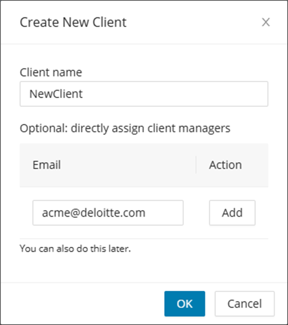
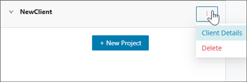
The client name card is created and you are now ready to create projects. To access the client details or delete the client entry, access the drop-down menu.
Create a project
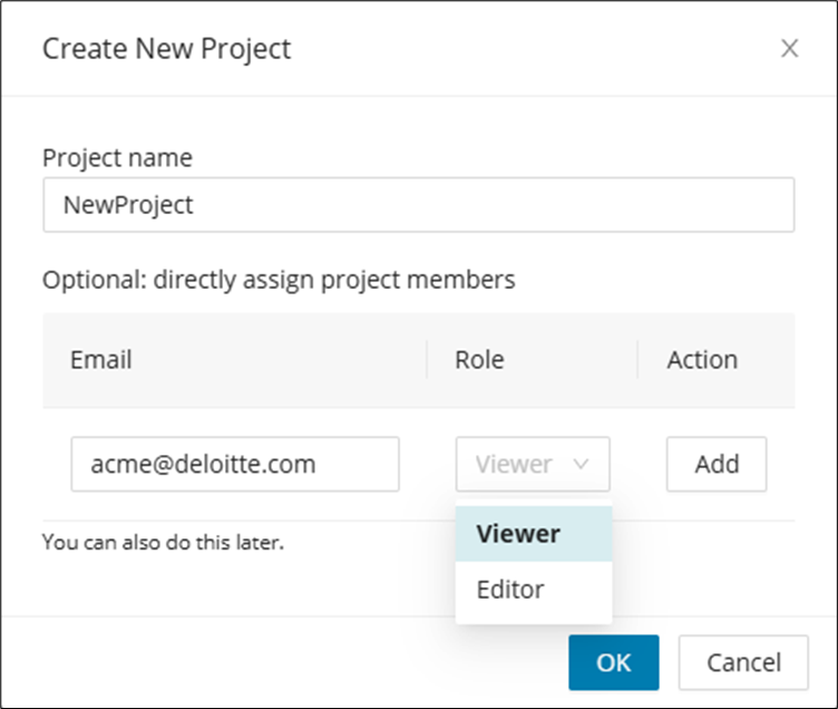
Click + New Project from the client name card and enter the project name and, if applicable, the project member details. You can choose either the "Viewer" or "Editor" role of each project member. Then click Ok .
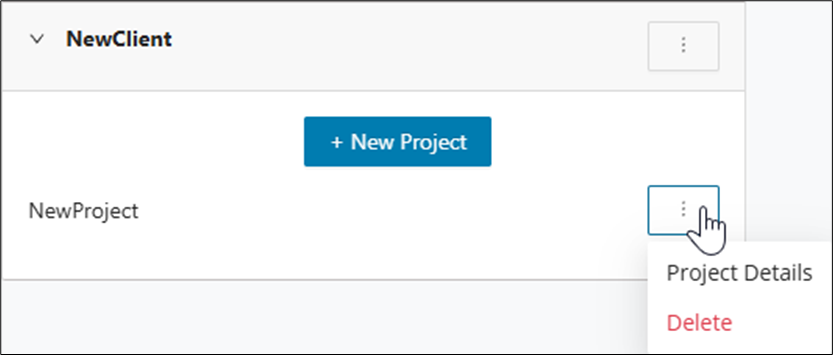
The project is created under the client name card with a menu to access the project details or delete the project entry. Click on + New Project to create additional projects under the same client.
Preparing your data for Decompose
Before you begin working with Decompose, you will need to have application data ready for analysis. The right preparation path depends on whether you already have Mining output or still need to assemble the source inputs. Use the guidance below to choose the starting point that matches your project situation.
-
Users with Mining Data: If you already have data extracted using Mining, you can proceed directly to importing this data set into Decompose. Simply follow the Import Process guide, which outlines how to load mining output and prepare it for analysis.
-
Users without Mining Data: If you do not have extracted mining data, please start by gathering your application source code or relevant data sources as outlined in the Data Preparation Guide. You may also initiate a mining process using Mining or prepare your own structured data sets according to the input specifications.
Both user types will find step-by-step instructions in the next sections to ensure a seamless onboarding and analysis experience with Decompose.
Imports
The Imports feature in Decompose provides a dedicated area for bringing multiple types of project data into the platform. This section is organized into tabs, allowing you to easily import schemas, modules, queries, taxonomies, and more. All of these are essential for analyzing and modernizing your legacy applications. Each import tab is tailored for a specific data type or purpose, streamlining the setup process for your project. Once your data is imported, you can take full advantage of Decompose’s powerful features, including decomposition, analysis, visualization, and database migration tools.
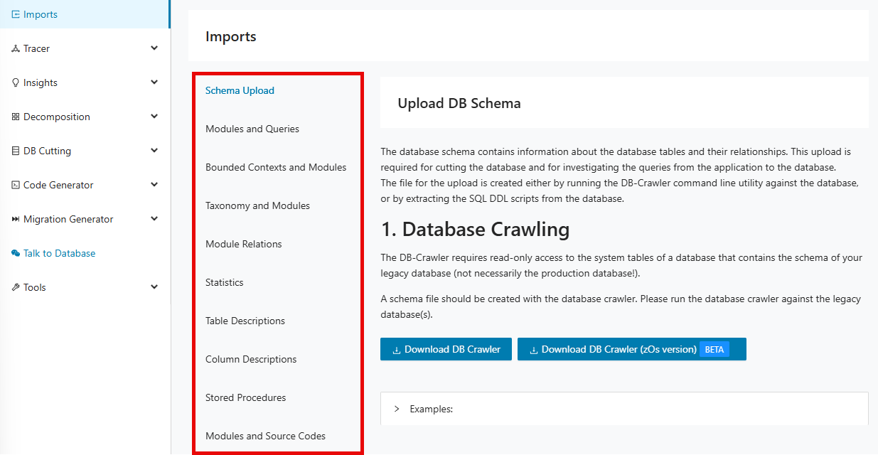
Import tabs
Info
The schema json file is present after crawling the database as a pre-requisite.
The database schema contains information about the database tables and their relationships. This upload is required for cutting the database and for investigating the queries from the application to the database. The file for the upload is created by running the DB-Crawler command line utility against the database.
Navigate to the "Imports" page from the left panel.
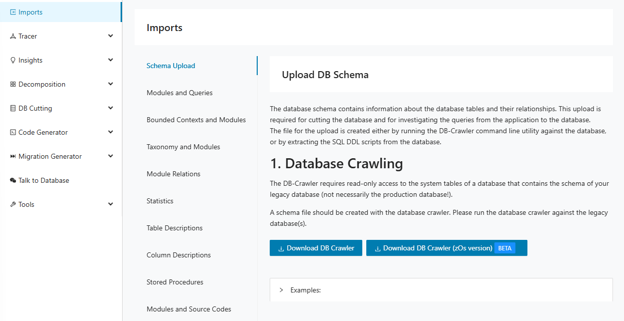
For a first time login, the user might not have the schema file and needs to extract it using the crawler. Download the crawler jar.
If the database is running in zOs click on Download DB Crawler (zOs version) Beta.
Otherwise click Download DB Crawler .
For more information on crawling, please refer to DB Crawling
Step 3:
Upload a json-file that has been created by DB Crawler or a SQL-file containing the DDL of the database (drag and drop the file into the upload area or click).
ADB2 generated reports
Decompose supports ADB2 generated reports. These can be imported in the same way as any other JSON file. Simply perform the steps from Schema Upload
The module import is required for all operations of the Decompose. The import file is generated from Code Discovery & Mining.
Step 1:
Navigate to the "Modules and Queries" tab then click Choose File .
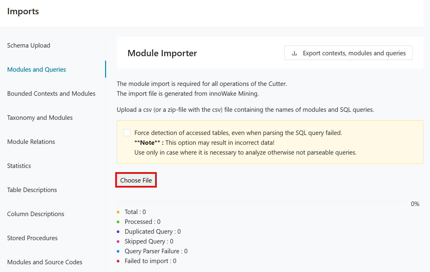
Step 2:
Browse and select the modules and queries file extracted from mining.
Simplify import errors
When importing the modules and queries, some queries may fail to parse or are skipped. Some of the simple questions the user may need to answer immediately are:
-
Which tables are missing? (Possibly also available from Mining if we also import the schema into Mining, but since we are providing an error list here, we might as well include it.)
-
What additional schemas need to be included?
-
What percentage of queries were successfully imported per module?
To get this information, the user must download the detailed error file.
This downloads a detailed_import_errors.xlsx file containing the error details during the query import.
It contains information about the schema, table/view, column and reason for the failures.
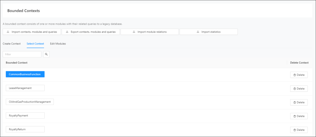
A Bounded Context defines the affiliation of modules to a domain. Each Bounded Context can be modernized separately, for example, into a Microservice or a cloud native application. The import file can be created by the Decompose itself. The import is completely optional, as Bounded Contexts can be generated from Taxonomies within the Decompose. Bounded Contexts can be exported from Mining. as well. This below steps describes how to import the bounded contexts exported from Mining.
Step 1:
Navigate to the "Bounded Contexts and Modules" tab then click Choose File .
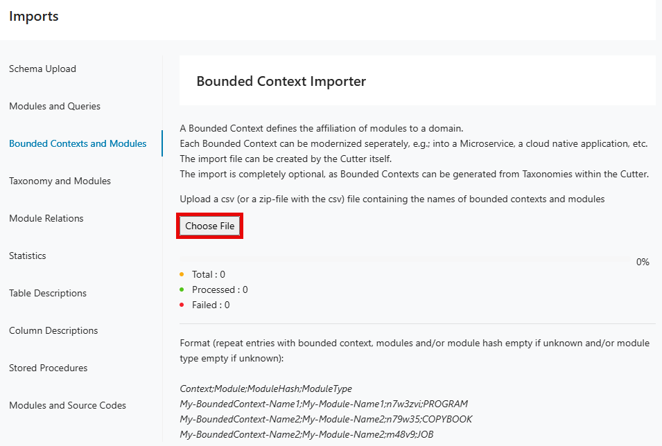
Step 2:
Browse and select the bounded contexts and modules file extracted from mining.
A taxonomy is a tag that can be attached to any module. Each module can have a multitude of assigned taxonomies. Taxonomies can be used to decompose an application. The import file can be generated by Mining. As Decompose itself can generate taxonomies, the upload is optional. The below steps describes how to import the taxonomies exported from Mining.
Step 1:
Navigate to the "Taxonomy and Modules" tab then click Choose File .
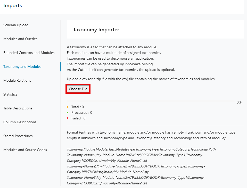
Step 2:
Browse and select the taxonomies and modules file extracted from mining.
The module relations import is recommended for all operations of the Decompose. The relations define the call chain between methods inside modules. The import file is generated from Mining.
Step 1:
Navigate to the "Module Relations" tab then click Choose File .
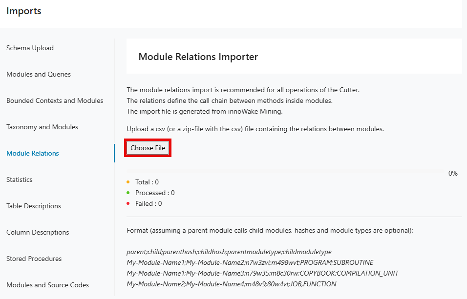
Step 2:
Browse and select the module relations file extracted from mining.
The statistics of a database indicate for example performance issues, tables with heavy load or large data sets. This import is completely optional and only needed for analysing the database in detail.
Step 1:
Navigate to the "Statistics" tab then click Choose File .
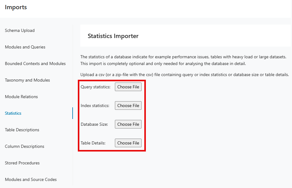
Step 2:
Browse and select the statistics file.
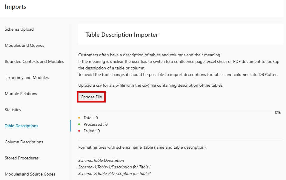
Customers often have a description of tables and columns and their meaning. If the meaning is unclear, the user has to switch to a Confluence page, Excel sheet or PDF document to lookup the description of a table or column. To avoid the tool change, it should be possible to import descriptions for tables and columns into DB Cutter.
Step 1:
Navigate to the "Table Descriptions" tab then click Choose File .
Step 2:
Browse and select the table descriptions file.
Customers often have a description of tables and columns and their meaning. If the meaning is unclear, the user has to switch to a Confluence page, Excel sheet or PDF document to lookup the description of a table or column. To avoid the tool change, it should be possible to import descriptions for tables and columns into DB Cutter.
The CSV format is as follows: Schema;Table;Column;Description
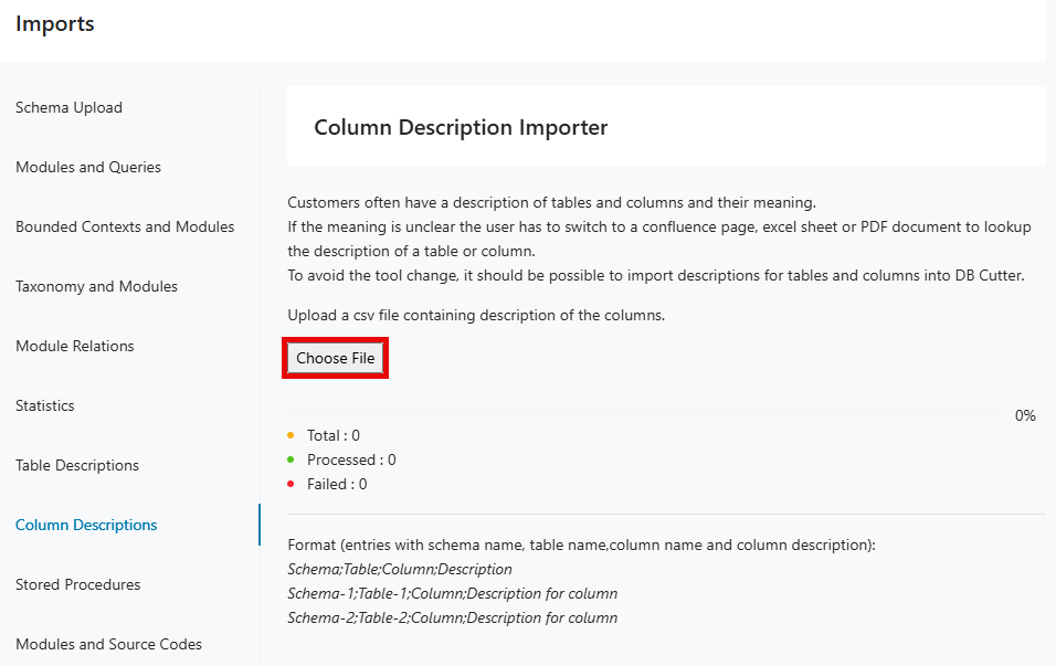
This can be verified and seen through Talk-to-database by search inputs like: "What is the purpose of START_TIME column?".
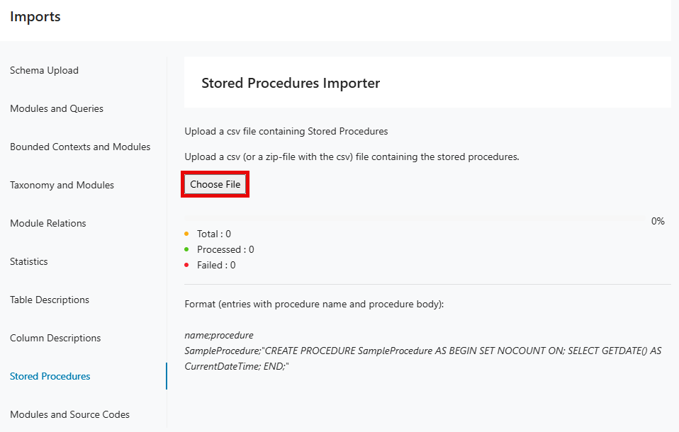
Upload a csv file containing Stored Procedures.
Step 1:
Navigate to the "Stored Procedures" tab then click Choose File .
Step 2:
Browse and select the stored procedures file.
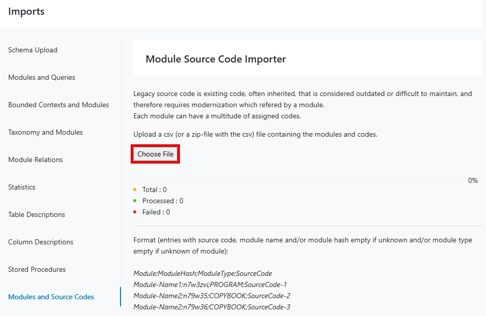
Legacy source code is existing code, often inherited, that is considered outdated or difficult to maintain, and therefore requires modernization which referred by a module. Each module can have a multitude of assigned codes.
Step 1:
Navigate to the "Modules and Source Codes" tab then click Choose File .
Step 2:
Browse and select the modules and source codes file.
Working with Decompose
Working with Decompose
The Decompose Web UI is organized into pages in the navigation panel on the left. Follow the links below to learn what each page does and how it supports the decomposition workflow.
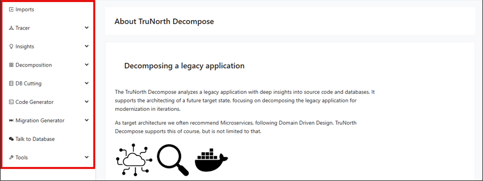
Navigation Panel
The navigation panel is the main entry point to the Decompose workflow and organizes features in the order most teams use them. Understanding what each page is for helps you move between import, analysis, decomposition, and modernization tasks without losing context. The table below summarizes the primary pages available from the left-side navigation.
| Page | Description |
|---|---|
| Imports | Import legacy application artifacts for deep source code and database analysis, kickstarting your decomposition journey. |
| Tracer | Dynamically trace user interactions and telemetry to uncover application behavior, providing vital context for decomposition. |
| Insights | Visualize relationships between code modules and database structures to inform architecture and modernization efforts. |
| Decomposition | Tag, group, and visually organize modules to iteratively break down your legacy application into meaningful sub-domains. |
| DB Cutting | Identify, segment, and remodel legacy databases, supporting the shift to modern, domain-driven data architectures. |
| Code Generator | Automatically generate modern database access code and service skeletons from legacy application and schema analysis. |
| Migration Generator | Generate detailed reports and tools to guide data migration from legacy systems to new target state databases. |
| Talk to Database | Interact with your database through an AI-powered conversational UI to quickly explore tables, columns, and relationships. |
| Tools | Access a suite of powerful utilities for analysis, transformation, and reporting throughout your modernization journey. |
About Decompose
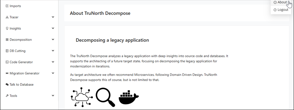
After creating your client and project, the first page introduced by Decompose is "About Decompose". Before diving into the application, take a moment to read through "About Decompose" to see how these tools and insights work together to guide your journey from legacy to modern architecture. You can always navigate back to "About Decompose" by clicking on About from the drop-down menu under the log-in info.
Tracer
Before you analyze and decompose an application, Decompose needs information about the application's internals. Besides static analysis, Decompose can also trace live interactions while people use the legacy application.
-
Instrumentation of the legacy application.
-
Analyzing telemetry data and log files.
-
Calculating taxonomies based on captured user actions.
-
Initial decomposition of the system.
The data that are collected by the Tracer are a good starting point for further analysis and decomposition, especially when there are no static code analysis data available.
Insights
Decompose identifies the relationships between source code and database tables/columns. Therefore it needs to know about:
-
Source code modules of the application.
-
The call chain between the source code modules.
-
The queries that are sent from the application to the database.
-
The database schema(s).
While the database cutter can work completely independent of other tools, it is recommended to use it together with our other products. Other products for static or dynamic source code analysis provide data about source code modules and their relationships. The integrated DB-Crawler reveals all necessary information about the legacy databases.
Decomposition
When working on large legacy applications, you usually do not want to modernize that with a big bang release. Instead you could want to modernize iteratively, moving parts of the old application to a new architecture and infrastructure.
Decompose will help you in doing so by offering a variety of options for decomposing your application.
-
You can create Taxonomies, for example, you tag a set of modules with a name.
-
You can automatically tag modules that belong together to a sub-application.
-
You can automatically tag modules that are accessing shared data.
-
You can visually edit taxonomies.
-
You can define sub-applications within your large legacy application.
In Domain Driven Design, these would be called domains, or Bounded Contexts. -
You can ask the Cutter to automatically split your application into domains.
Modernization
Decompose support the modernization of legacy applications and its databases:
-
Automatically define data for Bounded Contexts.
-
Analyze queries from the application to tables/columns in the database.
-
Design new databases for modernized parts of the old application.
-
Identify conflicts between Bounded Contexts.
-
Model interfaces between Bounded Contexts.
-
Generate reports for supporting the migration of data out of a legacy database into multiple target databases.
Generator
Decompose enables AI-supported source code generation from the collected knowledge about the database and the legacy application:
-
Generate the database layer for the modernized application, leveraging standard object-relational mappers.
-
Convert the SQL queries from your legacy database dialect to the SQL dialect of the desired modernized database.
-
Generate the repositories that use the generated queries.
-
Generate a service layer skeleton that leverages the generated entities, DTOs and queries.
Talk to Database
Decompose enables AI-supported discovery of your database assets, transforming collected knowledge about your database schema into an interactive, conversational experience. You can talk directly to the database by asking questions in natural language. Through the chat UI, you can ask "Give me details of TableA", "Show me columns of the table" and receive immediate, relevant answers from our GenAI-powered chatbot.
Insights
The Insights area helps you understand how legacy code and database structures relate to each other before you make decomposition decisions. It combines schema exploration, graph views, conflict analysis, and usage patterns in one workspace. Use these pages to validate assumptions and gather evidence for bounded context design.
Prerequisite
To use the Insights features, upload a valid schema .json file first. Create this file either by running the DB-Crawler command-line utility against the database or by extracting the SQL DDL scripts from the database.
Legacy Database
The Legacy Database feature provides a centralized interface for exploring the structure and contents of legacy database systems. This tab provides different comprehensive views of client's database to fully understand their database structure and schema.
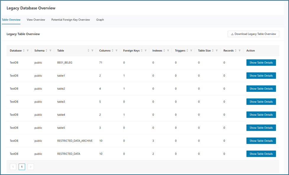
Table Overview
The Table Overview tab provides a clear summary of all tables within the selected database schema, supporting quick assessment and navigation.
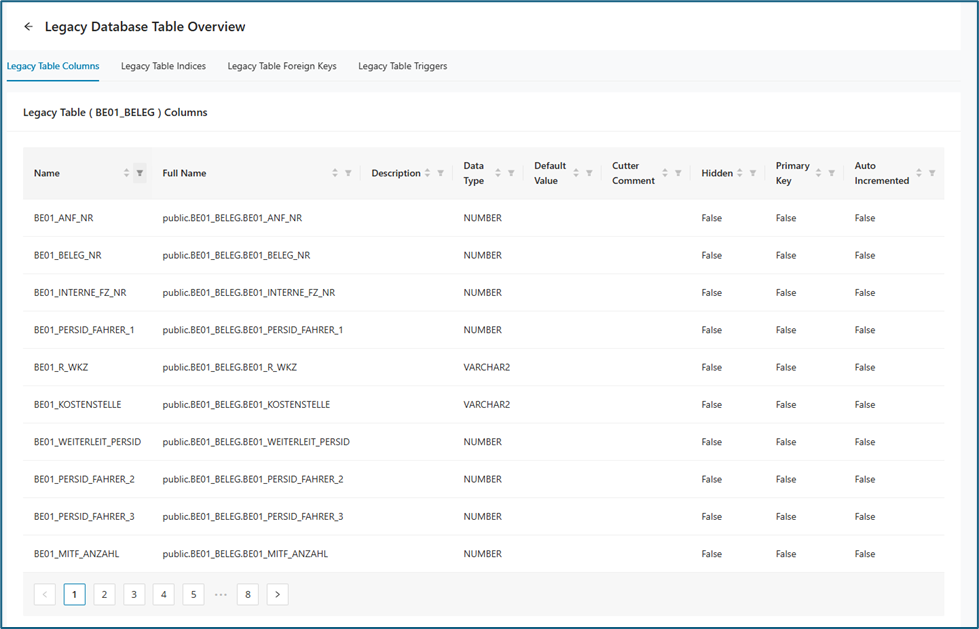
When Show Table Details is clicked, the system displays a detailed breakdown of the selected table’s columns, indexes, foreign keys, and triggers. Each category is presented in its own table, allowing users to easily review and understand specific aspects of the table’s structure.
View Overview
The Legacy View Overview table lists all the different views and the tables they are tied to. It also lists, for each view, the number of columns, indexes, and triggers associated with that view.
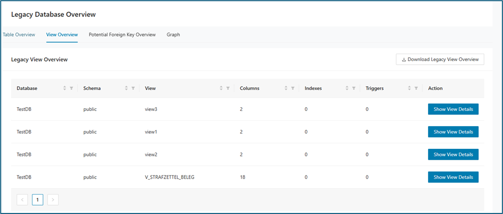
When Show Table Details is clicked, the page displays the characteristics of the selected view, such as column names, data types, sizes, and other relevant information. Additional details are available on the Legacy View Indices and Legacy Table Triggers tabs, if such information exists.
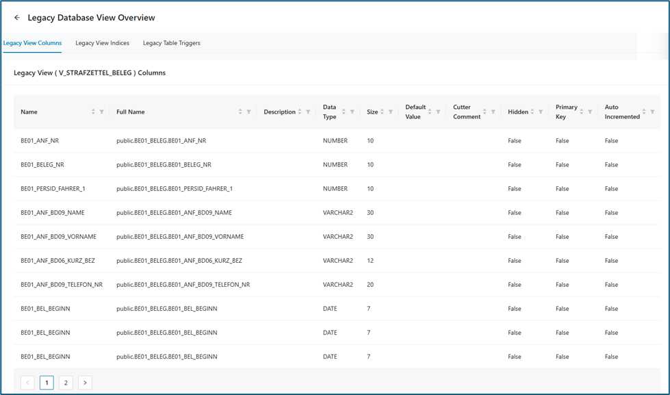
Potential Foreign Key overview
Graph
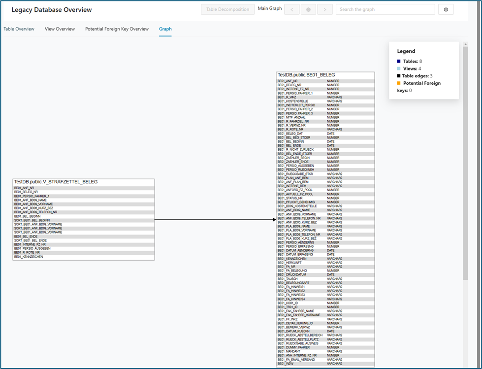
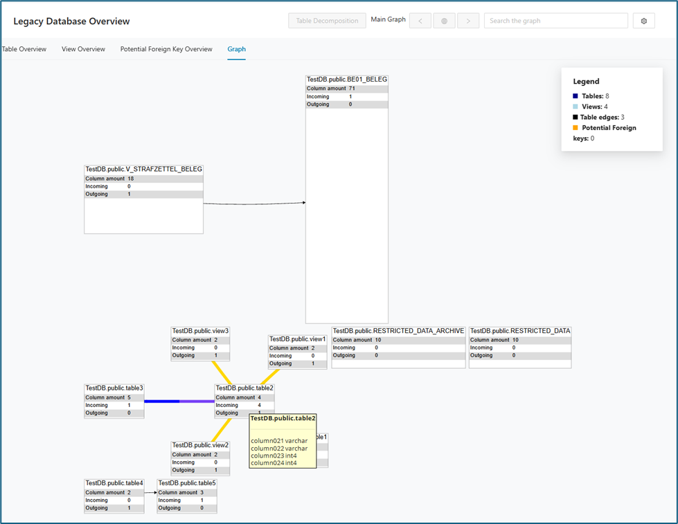
This graph provides a visual representation of the structure and relationships within your legacy database, as summarized in the Table Overview. It helps you understand how tables and views interact and highlights key relational features or gaps in the schema. The legend in the upper left corner of the Legacy Database graph displays the object count for the:
-
Number of Potential Foreign keys
-
Number of Tables
-
Number of Views
-
Number of Foreign keys (= edges)
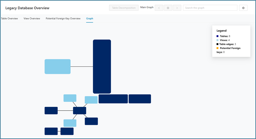
As you zoom in on the graph, additional details become available. The graph displays full names and shows how data flows into and out of each table and view.
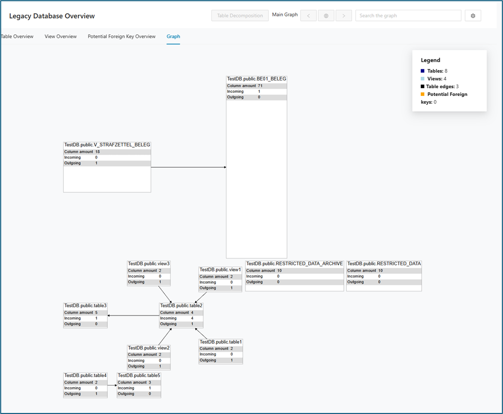
When you zoom in further, each table and view is shown with its full name, total number of columns, and the direction of incoming and outgoing links. For tables, all column names and data types are displayed, making it easy to review the schema details and relationships.
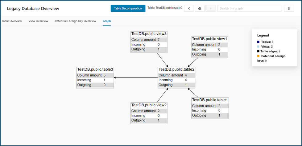
You can also click a specific table to focus the graph on that table and its related views.
Graph options
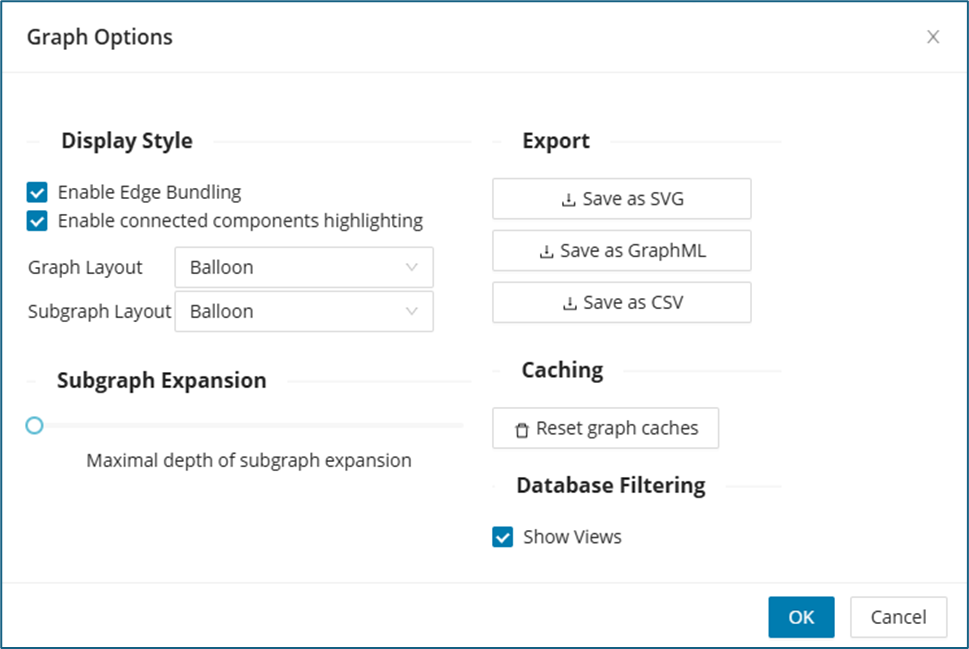
Users have flexible options to tailor the Graph/Subgraph Layout to their needs. Click the settings icon located in the top right to open the "Graph Options" window. Users can switch between different visualization styles, such as Balloon, Hierarchical, Organic, or Radial layouts, to best highlight the relationships among tables and views. The Subgraph Expansion slider allows you to adjust how many layers of related objects are displayed, controlling the depth of the graph for focused analysis or a more comprehensive view. Additionally, filtering options make it easy to customize what you see—for instance, you can hide views by unchecking the Show Views option, so only tables are displayed. These features help users explore the database structure in the way that best fits their specific analysis or troubleshooting task.
The Export feature makes it easy for users to download the current graph view in different formats. Users can choose to export the visualization as an SVG for high-quality images, as GraphML for further analysis in other graph tools, or as a CSV to capture detailed tabular data about the tables, views, and their relationships.
Query Paths
The Query Paths page shows the relation between source code and tables. Bounded contexts are represented by a diamond shape. Each context has its own color. Modules are represented by circles. If they are related to only one context, they take the color of the context. Tables are represented by gray squares.
The Query Paths graph shows the relationships between bounded contexts, modules, and tables. With this graph, you can see which modules access which tables, or view the same relationships from the table perspective. The graph supports zooming, filtering, and navigation to subgraphs.
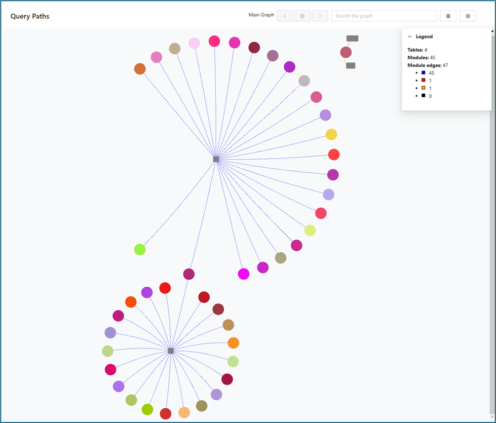
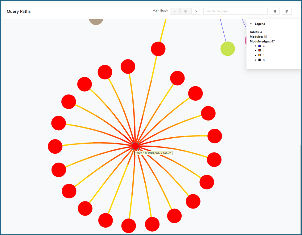
When the user hovers the mouse over a particular table in the diagram, all the connections between that table and associated modules are visually highlighted to indicate their relationships.
When a user clicks on a specific table, the graph will display the names and details of both the selected table and all related modules.
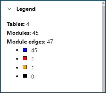
The color of each connection line represents the type of interaction between the module and the connected table:
-
Blue : The module reads data from the table
-
Red: The module has write access to the table.
-
Orange: The module has both read and write access to the table.
-
Black: The module triggers actions or processes related to the table (such as executing a stored procedure or initiating a workflow).
Here are few examples:
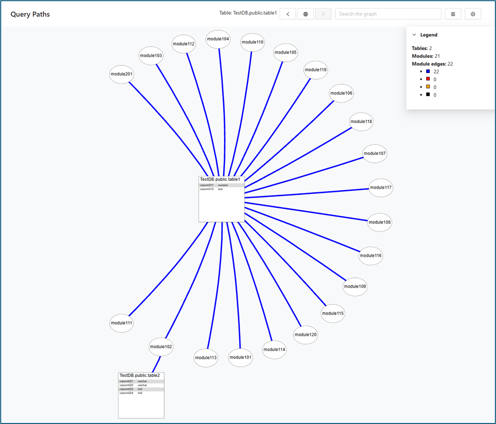
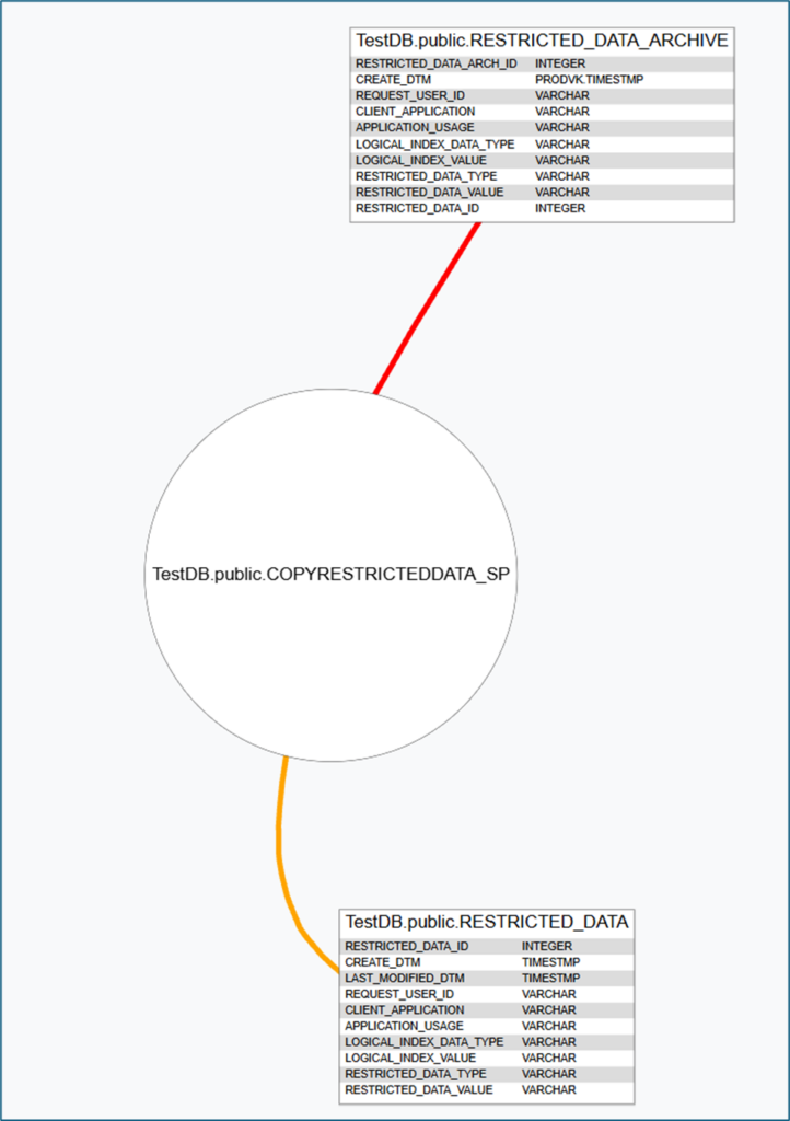
Object count in graph view
The legend automatically updates to reflect only the connection currently visible in the graph, adapting in real time as users filter or adjust what is displayed on the query page. The legend in the upper left corner of the Query Paths graph displays the object count:
-
For each bounded context:
-
Number of accessed tables
-
Number of modules
-
Number of queries
-
-
Number of unassigned modules
-
Number of queries in unassigned modules
Conflicts
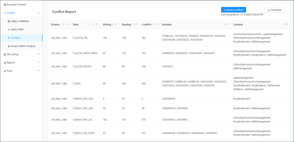
The Conflicts page contains information about the conflicts detected by the Decompose. The queries from each context accessing a column can be reviewed here.
The general workflow is to first import the database schema and then the csv file with the bounded contexts, modules and queries.
To analyze the conflicts in the database, navigate to Insights -> Conflicts and click Compute Conflicts in the upper right corner.
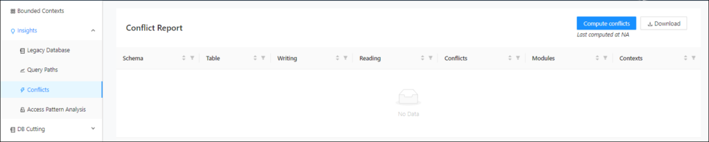
This will start a background task to calculate the conflicts, after which the conflicts will be displayed on the page. This way, the data doesn’t have to be recomputed for each filter/sort operation all over again.
Access Pattern analysis
Use Access Pattern analysis to evaluate how tables and columns are used in application queries before you choose a target data design or database technology. The view highlights which columns are used as access conditions in WHERE clauses and JOIN conditions, which is especially important when you compare modernization options for technologies with stricter and more expensive indexing constraints such as DynamoDB. Use the results to understand how read, write, and filter behavior may influence your target-state decisions.
To see the Access Pattern Analysis features, create a project, upload a valid dbcrawler JSON file, and then upload a valid CSV file in Import contexts, modules and queries under Bounded Contexts.
Query Analysis
Use the search bar to find a table name, for example- table public.RESTRICTED_DATA_ARCHIVE. It shows an overview of the columns of the table used in a WHERE clause or a JOIN condition categorized by SQL statement type (SELECT, UPDATE, DELETE).
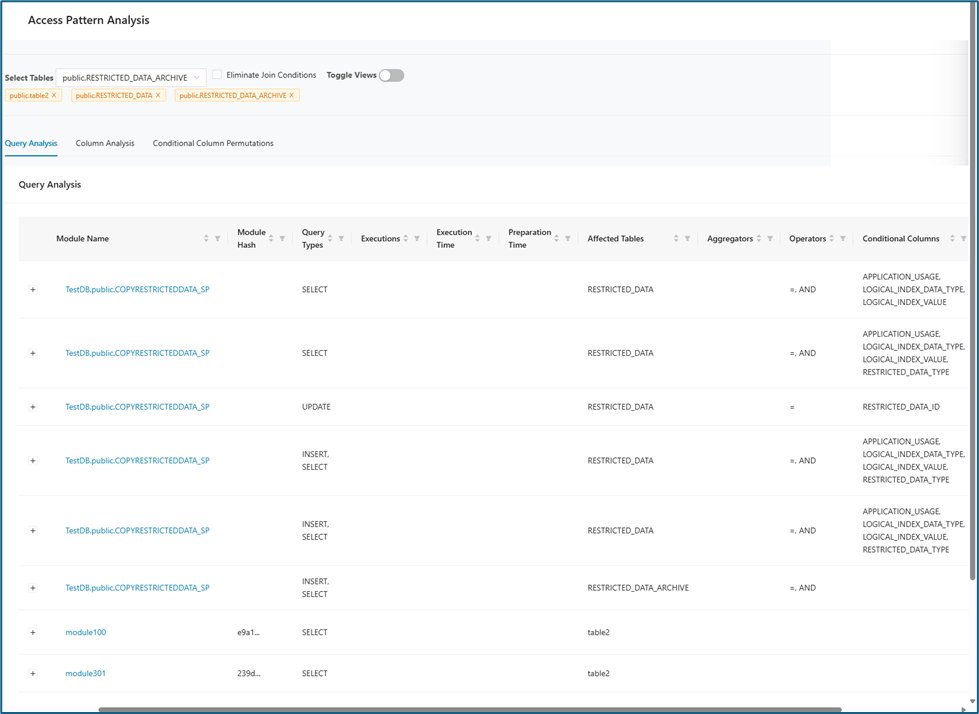
The following table describes the various table headers and their definitions:
| Table Header Name | Description |
|---|---|
| Module Name | The module name to which the query belongs. |
| Module Hash | This is a unique identifier (usually a short alphanumeric string generated by a hash function) for a specific version or state of a code module, stored procedure, or script. |
| Query Type | Type of query. These can be either DELETE, SELECT, INSERT, or UPDATE. |
| Executions | The number of executions of a query in a DB2 database. |
| Execution Time | The execution time in a DB2 database. |
| Affected Tables | The table(s) affected by the query. |
| Operators | The operators used in a query like =, >, etc. |
| Conditional Columns | These columns are within a table or query that are used in WHERE clauses, JOIN conditions, or other logical filters (for example, WHERE COLUMN_A = 'XYZ'). |
| Bounded Context Name | This column indicates the bounded context(s) associated with the module, showing which specific domain areas or functional boundaries within the system the module is part of. |
Column Analysis
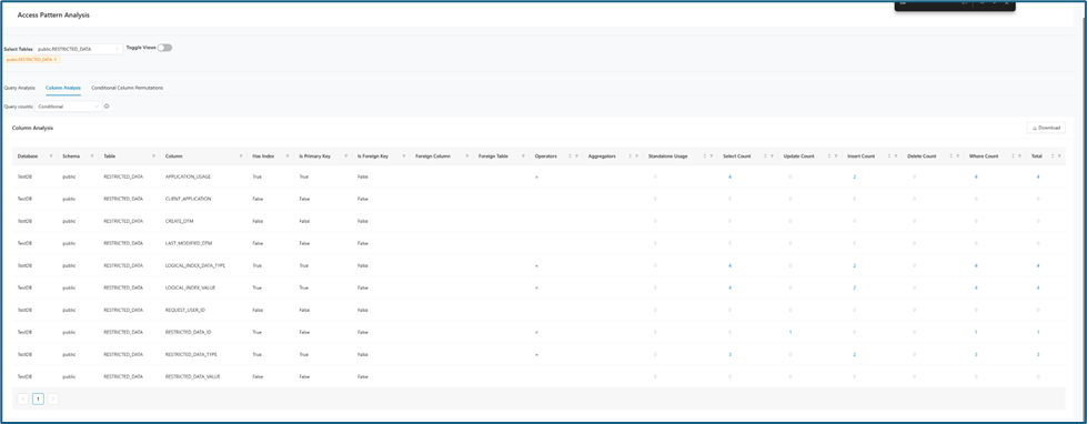
Within the Column Analysis tab, you can click any numerical value that appears as a hyperlink. Doing so reveals detailed information about the associated SQL commands such as SELECT, UPDATE, INSERT, DELETE, and WHERE clauses for that column.
The Column Analysis view has been enhanced with the addition of the Where Count column, which accounts for the usage patterns or counts of columns used in the "WHERE clause" of SQL queries. This data point is crucial from an architectural standpoint and for understanding the usage of a column or attribute from the legacy code perspective. This enhancement provides a more comprehensive view of column usage, similar to the existing metrics for Select count, Update count, and Delete count.
The Query Counts drop-down menu offers three options:
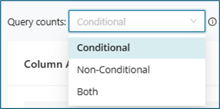
| Option | Description |
|---|---|
| Conditional | Displays queries containing conditions such as the “WHERE” clause for the column. |
| Non-Conditional | Displays queries without conditions for the column. |
| Both | Displays queries both with and without conditions for the column. |
This table provides detailed information about the names and descriptions of each column in the Column Analysis table:
| Table Header Name | Description |
|---|---|
| Table | The content can be filtered by conditions related to the table name. |
| Column | The content can be filtered by conditions related to column name. |
| Has Index | The content can be filtered by True or False. |
| Is Primary Key | The content can be filtered by True or False. |
| Operators | The content can be sorted and filtered by operators. |
| Aggregators | The table content can be filtered by data-gathering aggregators. |
Count column analysis
For this example, the number 4 was clicked in the first row under the Select Count column:
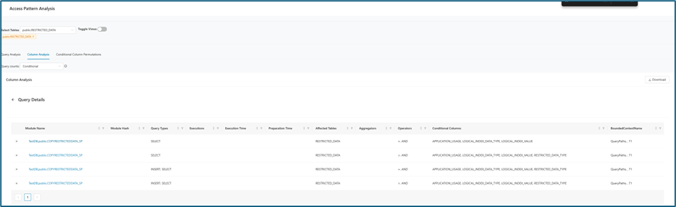
The query details are organized in a clear, tabular format. If you click a module name in this table, the interface redirects you to the corresponding page within the Mining project. That page provides detailed documentation, analytics, and related information about the selected module.
You can run the same analysis for the other columns.
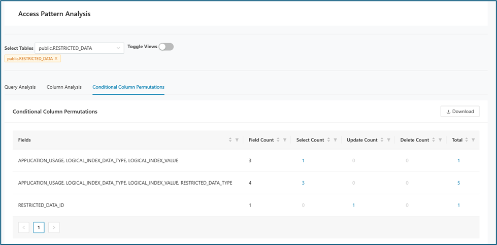
Conditional Column Permutations
Permutations shows how columns depend on each other. It lists the queries in which those columns are used together in the WHERE clause and helps you understand the dependencies that matter for database cutting.
Reports
This section holds different reports related to the Insights module. All reports could be downloaded as a .csv file.
Module List
The Module List provides a comprehensive table displaying all modules, including key details such as Name, Module Hash, Path, Module Type, and whether each module is Omitted in Graphs. For added convenience, a direct link to the mining project is also available. Below is a sample screenshot illustrating the module list layout.
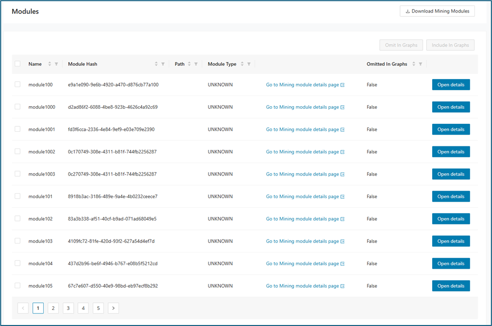
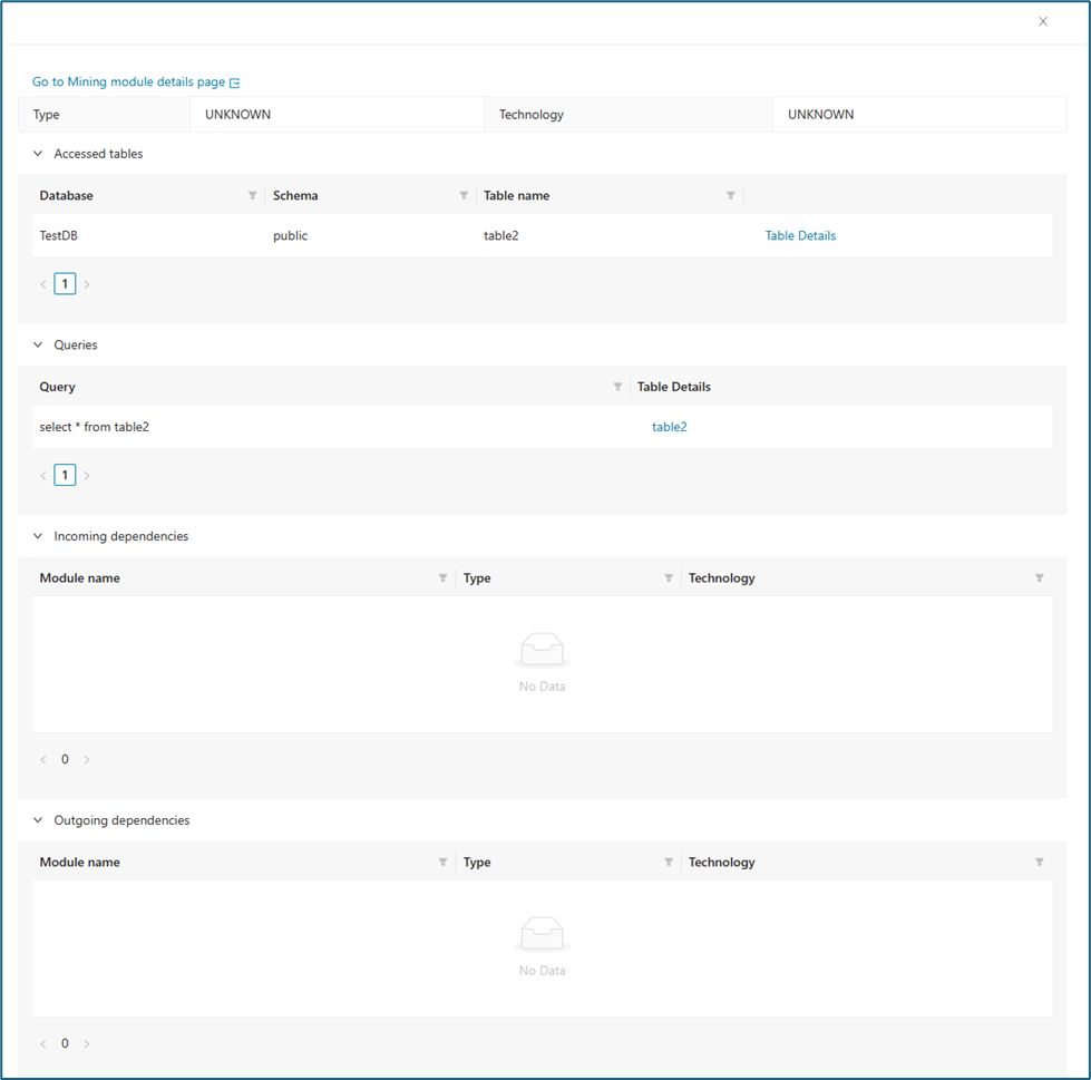
Open Details shows the module relations and the link to the Mining UI.
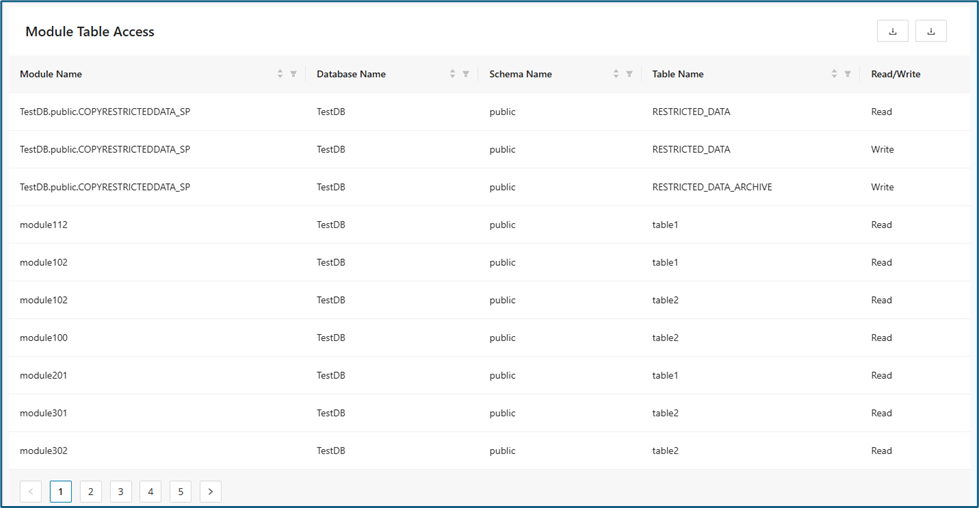
Module Table Access
The Module Table Access section displays a detailed table summarizing which database tables each module can access. Each entry includes the Module Name, Database Name, Schema Name, Table Name, and the corresponding access level (Read or Write). This organized view provides clarity on data permissions across modules.
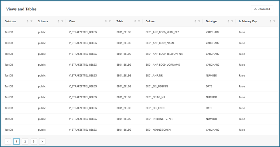
Views and Tables
The Views and Tables section presents a detailed overview of all database views, tables, and their attributes. It lists each view alongside information such as the associated table, column name, data type, and whether the column is a primary key. This organized table enables users to quickly identify data structures and relationships within the database.
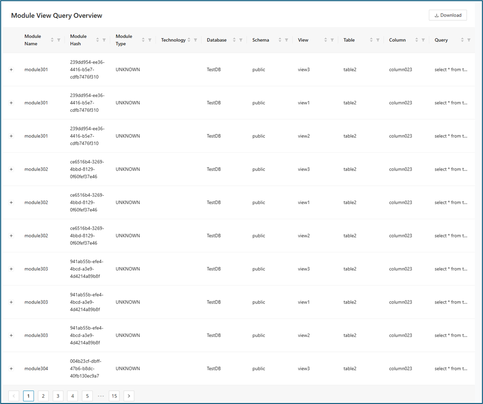
Module View Query
The Module View Query Overview section offers a detailed summary of the queries executed by each module. The table displays the Module Name, Module Hash, Module Type, Technology, Database, Schema, View, Table, Column, and the executed Query. Users can review which queries are associated with specific modules and gain deeper insights into data access patterns.
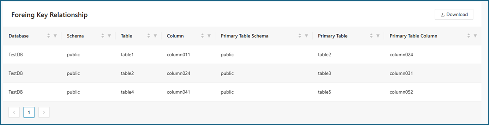
Foreign Key Relationship
This section provides a summary of foreign key relationships in the database. The table lists the database, schema, table, column, and their corresponding primary table and column, making it easy to trace data linkages across tables.
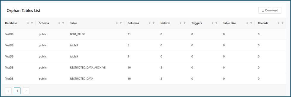
Orphan Tables
This section lists tables in the database that lack foreign key connections, showing their columns, indexes, triggers, size, and record count.
Decomposition
Decomposition
When you work with a large legacy application, you typically do not want to modernize it with a big-bang release. Instead, you modernize it incrementally by moving parts of the application to a new architecture and infrastructure.
Decompose supports that approach by providing several ways to decompose your application.
- You can create taxonomies by tagging a set of modules with a name.
- You can automatically tag modules that belong together to a sub-application.
- You can automatically tag modules that are accessing shared data.
- You can visually edit taxonomies.
- You can define sub-applications within your large legacy application. In Domain Driven Design, these would be called domains, or Bounded Contexts.
- You can use Decompose to split your application into domains automatically.
Feature overview
The Decomposition workflow is split across several focused pages, each supporting a different stage of grouping, analyzing, and refining candidate bounded contexts. Reviewing these pages in sequence helps you move from initial taxonomy work to graph-based analysis and reporting. Use the table below to choose the feature that matches your current decomposition task.
| Feature | Description |
|---|---|
| Taxonomy Editor | Create and refine taxonomies, manage modules, combine or intersect taxonomies, and assign taxonomies from endpoints, tables, and columns. |
| Reachability Analysis | Identify modules across call chains between upper and lower taxonomy boundaries and generate taxonomies from those paths. |
| Taxonomy Graph | Visually analyze taxonomies, their edges, shared resources, and graph-level editing actions. |
| Decomposition Wizard | Access the decomposition wizard section in the Decompose workflow. |
| Bounded Context Graph | Visualize bounded contexts, inspect relationships, and explore internal and external connections between modules. |
| Bounded Context Editor | Convert selected taxonomies into bounded contexts and manage taxonomy-to-context assignments. |
| BC Candidate Reports | Review candidate-edge, connection-summary, and access-pattern reports for bounded context candidates. |
| Reports | Review connected context, orphan module, and context query path reporting for bounded contexts. |
Taxonomy Editor
Use Taxonomy Editor to edit existing taxonomies or create new taxonomies by using Modules, Union, Intersect, Tag from endpoint, and related options. Taxonomies are usually created in Mining and assigned modules there, but Mining does not support building module chains from endpoints, columns, or tables. Taxonomy Editor lets you refine imported taxonomies or create new ones for microservice design.
Taxonomies tab
When you open Taxonomy Editor from the Decomposition section, the page opens on the Taxonomies tab. From there, you can view, create, edit, select, and delete taxonomies, and you can open the selected taxonomy directly in Taxonomy Graph.
The taxonomies are displayed together with description, category, type and action options as below.
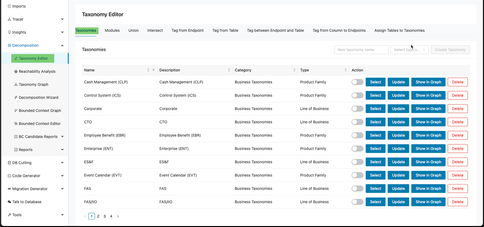
This information is loaded from the CSV files uploaded on the Import screen after you create a client and a project.
Each column supports filtering and sorting so you can narrow the results.
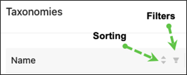
Creating a new taxonomy
To create a new taxonomy:
a. Enter an appropriate taxonomy name under the “New taxonomy name” text box.

b. Select the type under the “Select type of…” drop-down menu. Then select the appropriate choice.
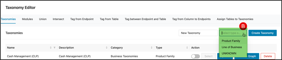
c. Finally, click Create Taxonomy.

Locate the the new Taxonomy from the Taxonomies table to verify the creation.
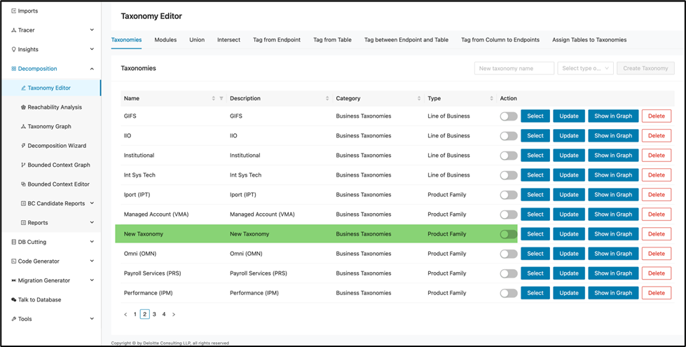
Select or configure a taxonomy
Once a taxonomy is selected, its structure will inform what modules and groupings you see and work within subsequent tabs (such as Modules).
First, click Select to select a taxonomy.
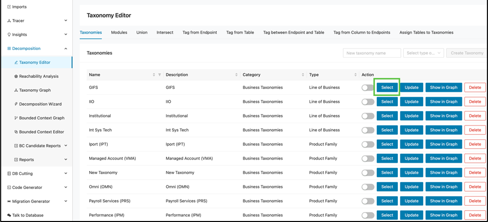
The Select button will be grayed out to indicate that the corresponding taxonomy has been selected.
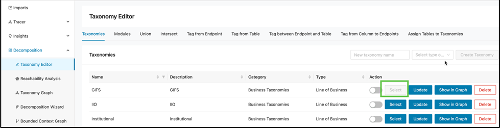
The selected taxonomy is reflected on other pages. For example, on the Modules tab, the taxonomy is selected automatically when you open the page for modules associated with that taxonomy.
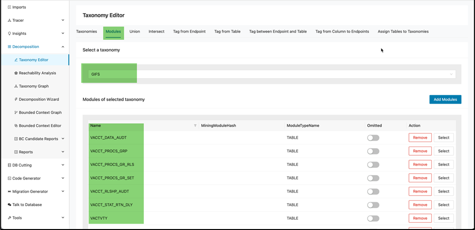
Selecting a different taxonomy on the taxonomies tab will unselect the previously selected taxonomy.
Updating a taxonomy
At times you may need to modify an existing taxonomy with a more appropriate description of business process.
Click Update to update a taxonomy.
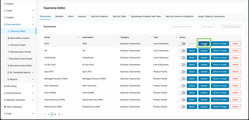
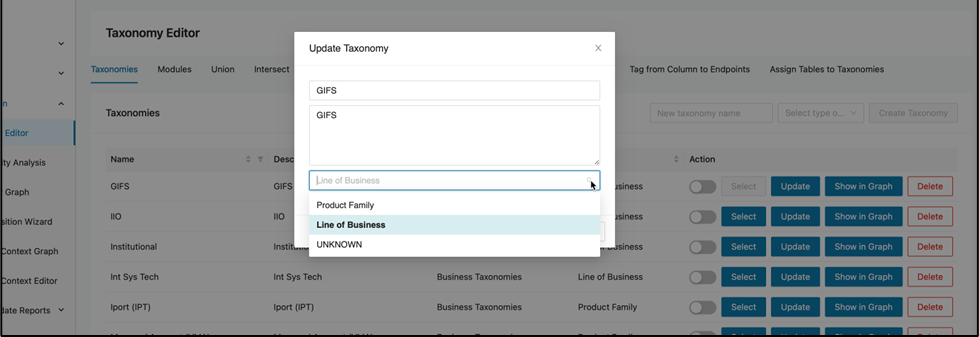
This opens a window for editing and saving changes. Edit and then click OK to save the changes.
Display graph of a taxonomy
Click Show in Graph to display the taxonomy in the graph.
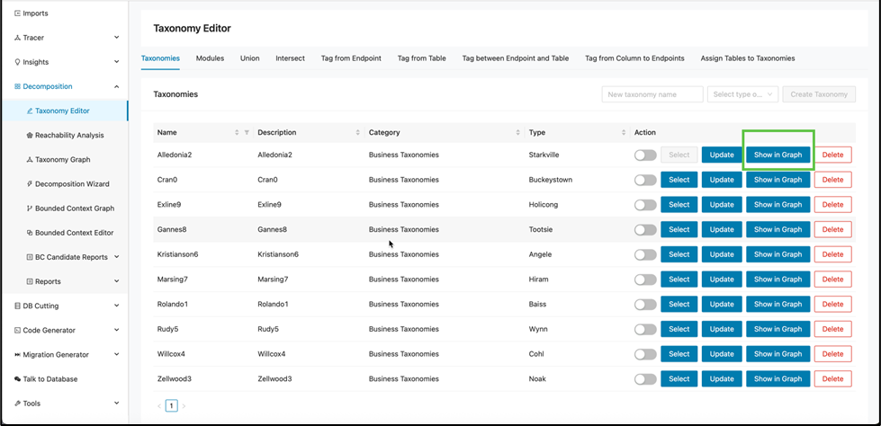
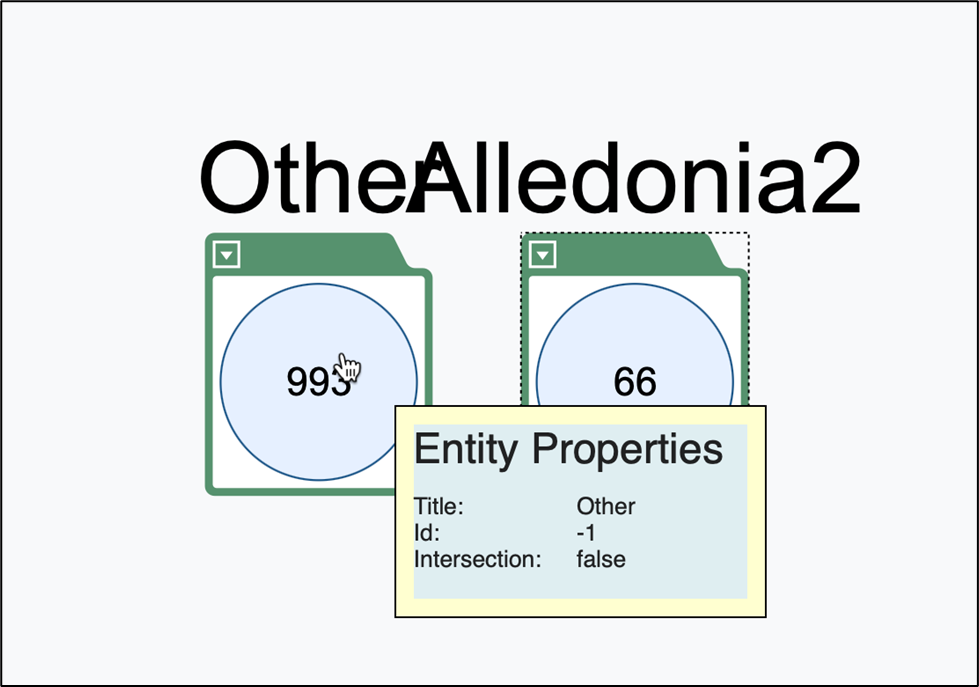
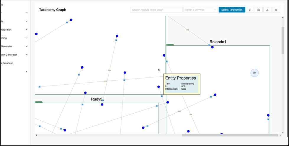
Afterwards, the “Taxonomy Graph” page will open and display the taxonomy you selected. You can also hover over elements within the graph to view the properties of each taxonomy:
-
The number of modules not expanded associated by circled number
-
Intersections: whether it be true or false
-
The title of the taxonomy
-
ID: is just for developers such as the DB ID
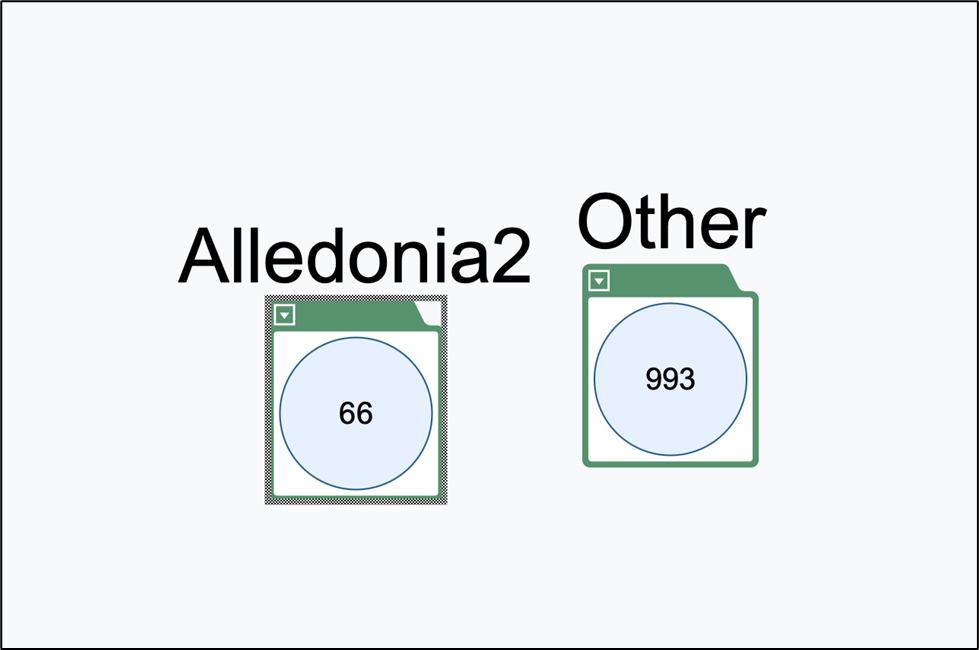
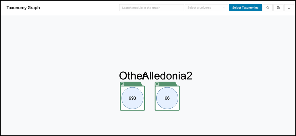
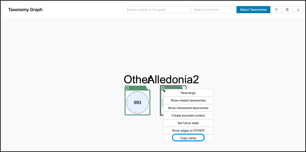
Below, the “Alledonia2” taxonomy is connected to “Other” taxonomy which in fact are other taxonomies in short. This is because we don’t want the graph to have a convoluted display. However, those taxonomies can be displayed.
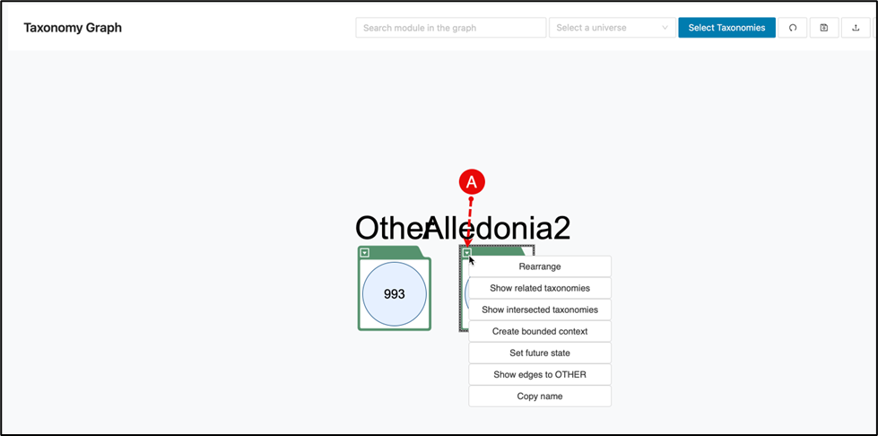
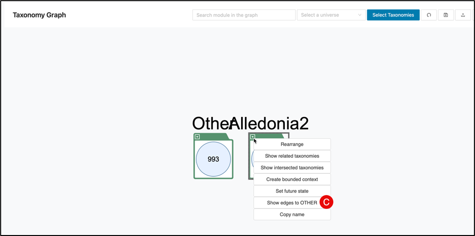
It is also normal for taxonomy names to overlap or blend in the visualization, but this can be corrected by doing the following.
a. Right click on your selected taxonomy.
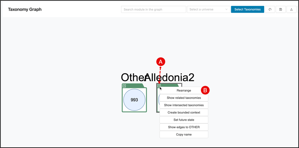
b. Rearrange: allows for the graph to be rearranged to a clearer view as below.
c. Show edges to OTHER: Will rearrange even further to show connected endpoints.
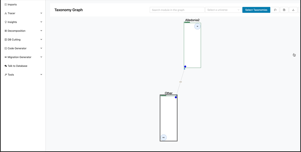
The graph layout can be customized by selecting a taxonomy and dragging it to your preferred position.
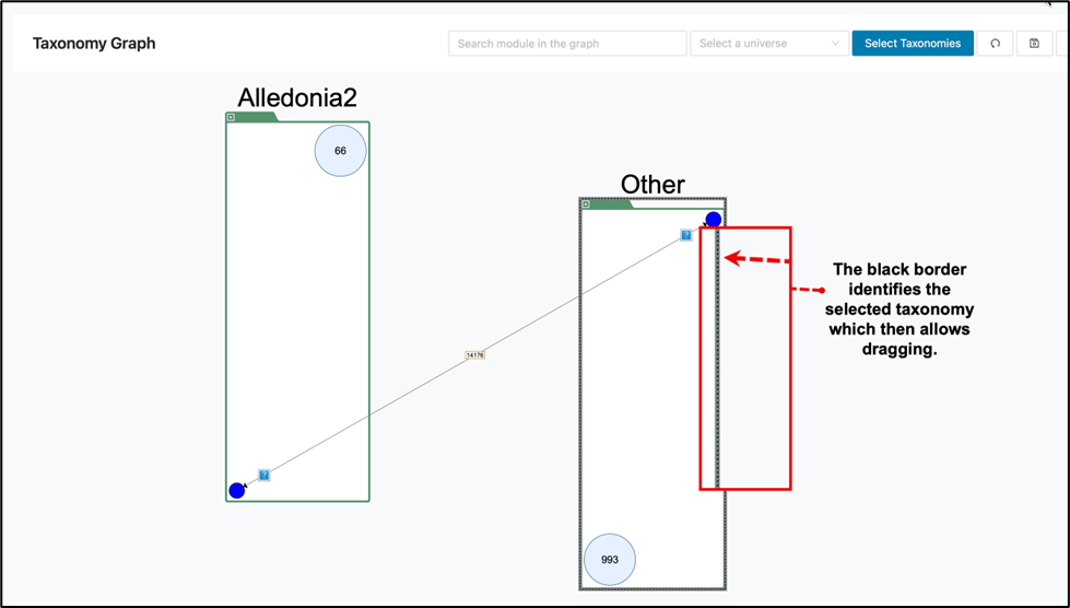
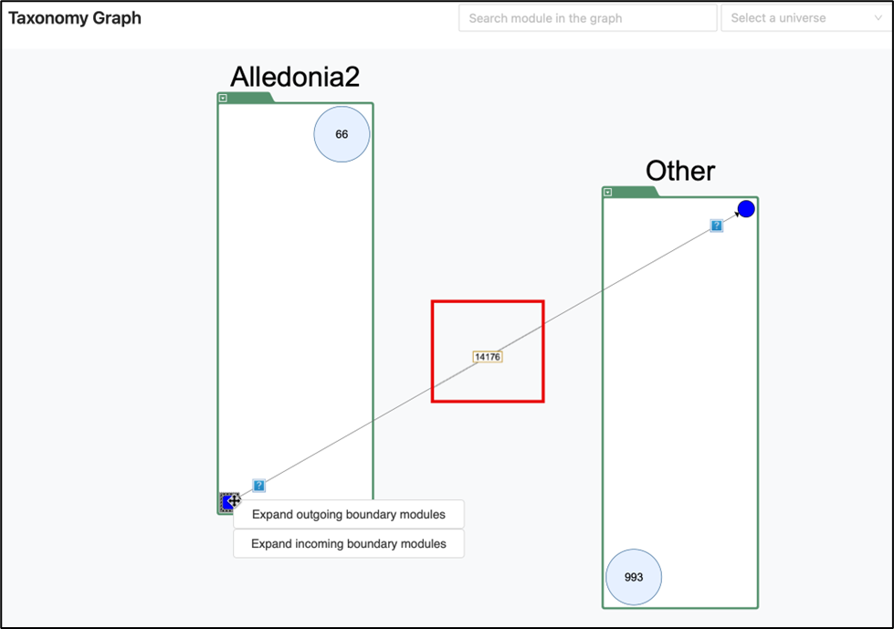
The "Show edges to OTHER” feature displays a blue dot on each taxonomy, which can be right clicked to access additional options. This view also highlights incoming and outgoing connections using arrows, and the total number of connections between the selected taxonomy and others is indicated by the magnified red box.
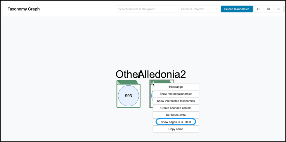
After clicking “Show edges to OTHER”, you can choose to expand outgoing or incoming boundary modules.
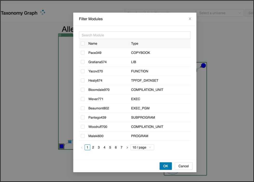
Be mindful of the number of modules within a taxonomy before expanding outgoing or incoming boundary modules, as this can make the view complex. If expansion is selected, a filter modules window will appear to help you limit and organize the display.
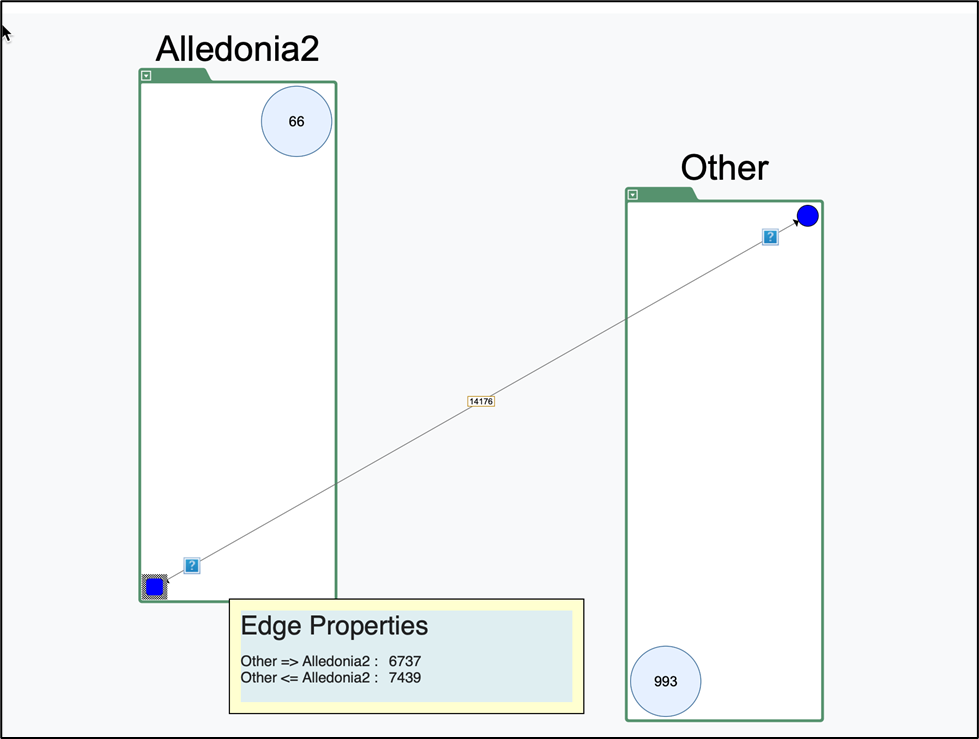
Edge properties
Hovering over the question marks on the connection arrow will display edge properties displaying the exact number of connections outgoing and incoming.
Other display options
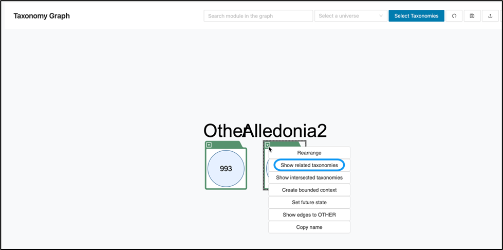
Again, to show other display options for a taxonomy, right-click the taxonomy.
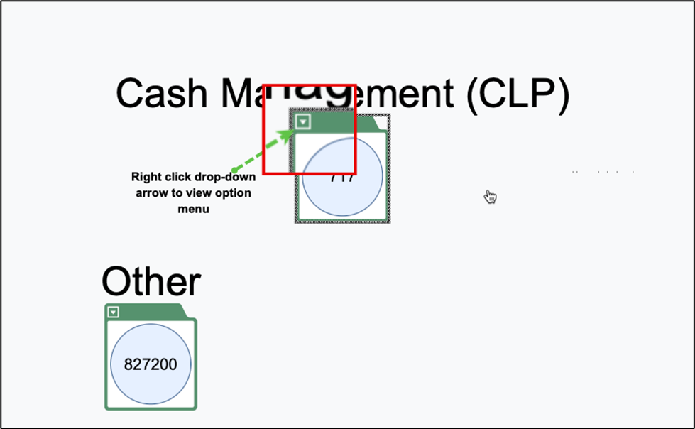
Show related taxonomies: will display a pop-up menu displaying related taxonomies not currently shown on the graph. By selecting any unrelated taxonomy from the table, you can instantly update the graph to include these elements.
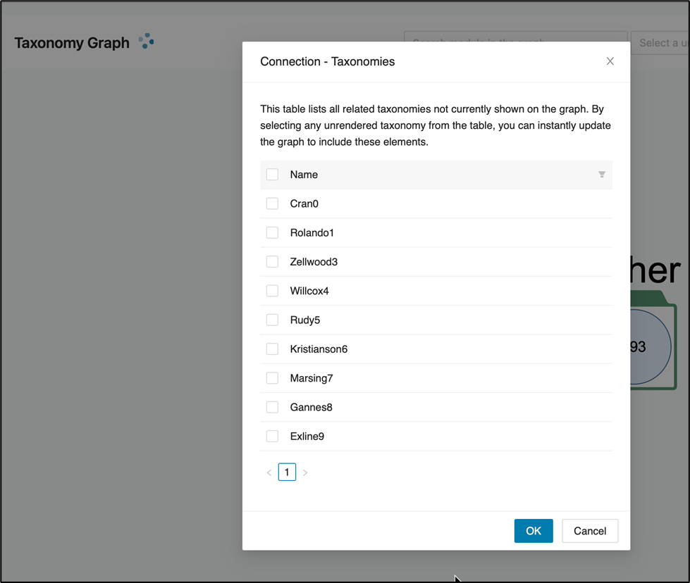
The example above only had 9 taxonomies so all nine were selected to display as below which gives you an idea on how to manage your displays.
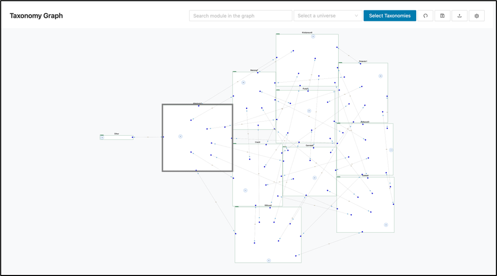
The operator can also enlarge a display with up and down dragging of your mouse.
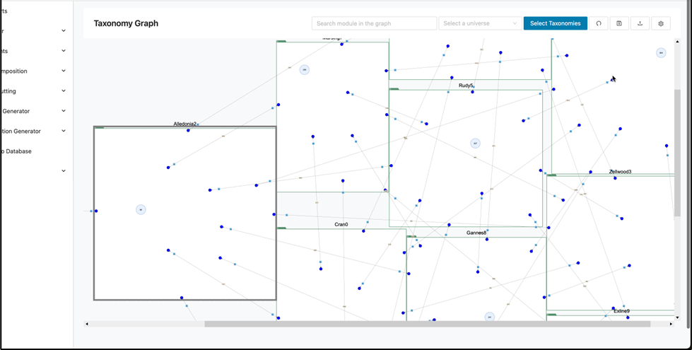
Left and right dragging of the mouse manipulates horizontal viewing.
Clicking out of the taxonomy graph menu to another menu and back will reset your view.
Show intersected taxonomies: When you hover over a taxonomy to view its properties, the interface will indicate whether it intersects with other taxonomies (intersection: true/false) as highlighted below.
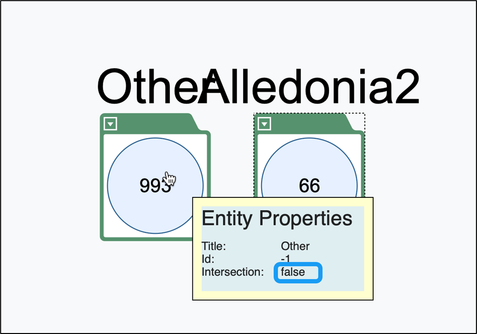
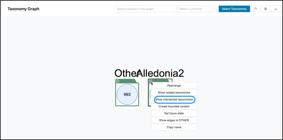
If intersection is false, selecting this option will display a banner stating, “The selected taxonomy does not have intersections with other taxonomies.”

If intersection is true, this means the selected taxonomy shares modules within it with another taxonomy. Displaying this intersection provides a clearer view of relationships within your system and may help identify opportunities to consolidate or harmonize related taxonomies.
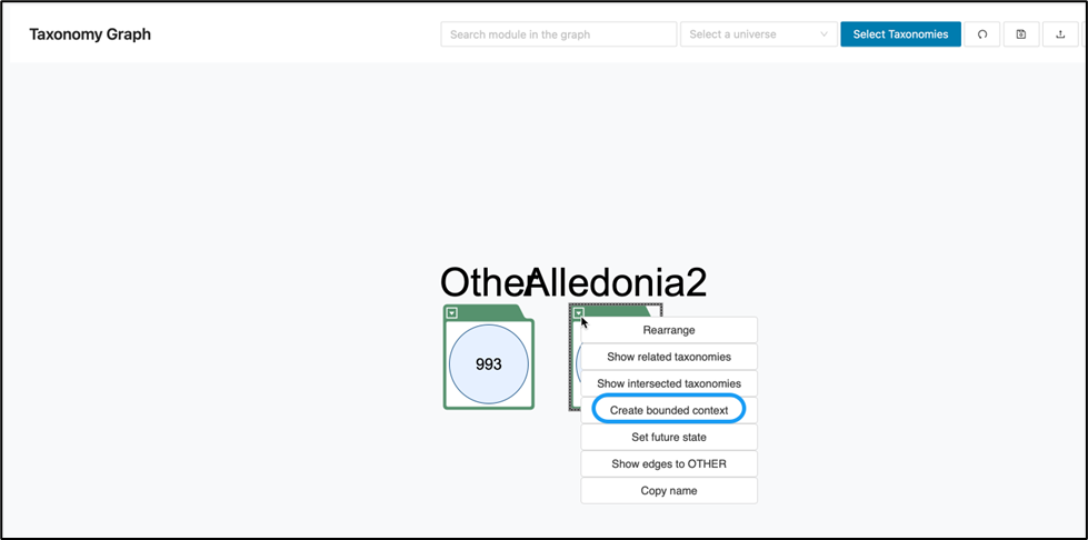
Create bounded context: Creates a new bounded context directly from the selected taxonomy node.
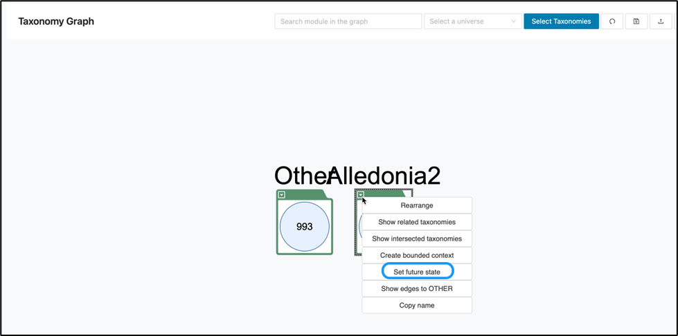
Set future state: Marks a taxonomy node with a future-state designation for planning and tracking architectural changes or migration paths.
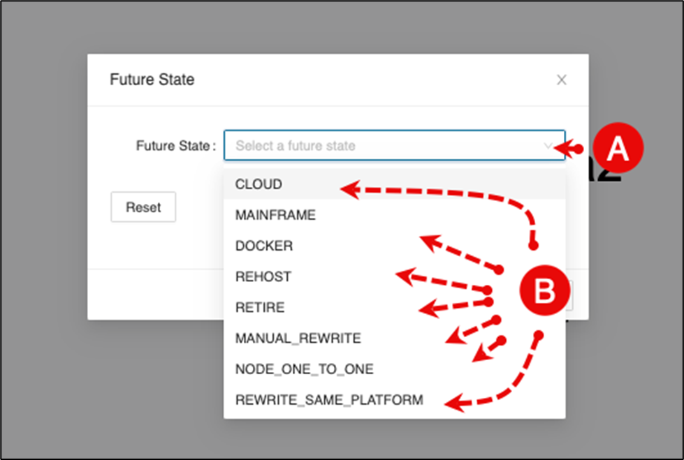
-
Click the drop-down arrow to select a future state.
-
Select a future state from the list.
Copy name: This option copies the name of the selected taxonomy node to the clipboard, making it easy to reference or use the taxonomy name in other contexts or documentation.
Deleting a taxonomy
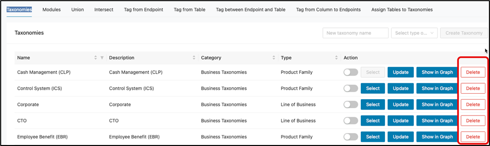
Deleting a Taxonomy will remove it from the Project. Click Delete within the Action column of a taxonomy. This action will remove an entire taxonomy and its associated modules from your project if it’s no longer needed so be mindful before doing this.
Modules tab
Modules are configurable components containing logic, rules, or data transformations that you can apply to taxonomies within the Decompose suite. The Modules tab lets you manage these building blocks to create flexible, reusable processing routines.
The most recently selected taxonomy in the Taxonomies tab automatically becomes the default selection in the Modules tab, together with all modules currently associated with that taxonomy. Within this workspace, you can:
-
Edit Taxonomies by Managing Modules: Add new modules or remove existing ones to customize how your taxonomy processes data.
-
Omit Modules from the Taxonomy Graph: Temporarily exclude specific modules from being represented in the taxonomy visualization for a cleaner or targeted view.
-
Render the Edited Taxonomy Graph: Instantly display changes and see how edits affect the structure directly within the Taxonomy Graph.
-
Delete a Taxonomy from the Project: Remove an entire taxonomy and its associated modules from your project if it’s no longer needed.
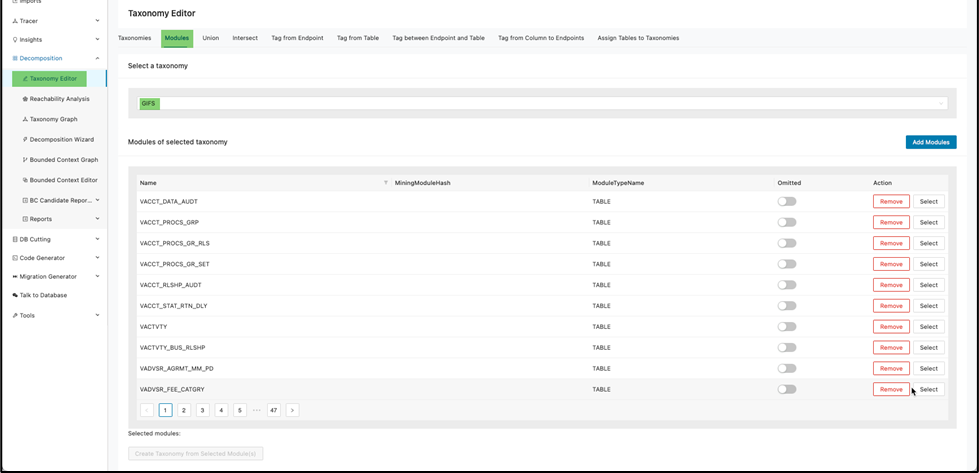
How to add modules to a taxonomy
To add a module within a taxonomy, start by ensuring the correct taxonomy is selected. You can do this in two ways:
a. Click the drop-down arrow in the “Select a taxonomy” search field under the Modules tab to choose from available taxonomies.
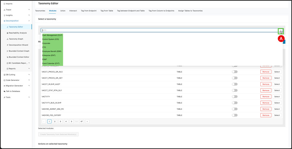
b. Select your desired taxonomy from the list.
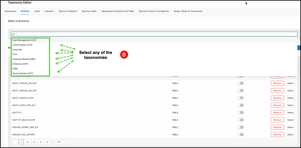
After a brief processing period, the Modules tab will display all modules currently associated with that taxonomy. For example, choosing the “Control System (ICS)” taxonomy may show hundreds of modules, organized 10 per page.
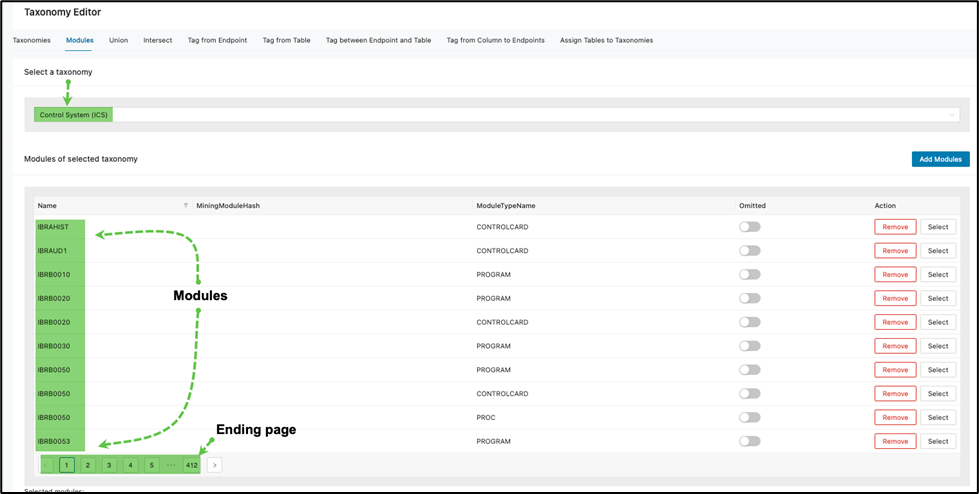
c. To add more modules, click Add Modules .

A pop-up window will appear, listing additional modules available for selection.
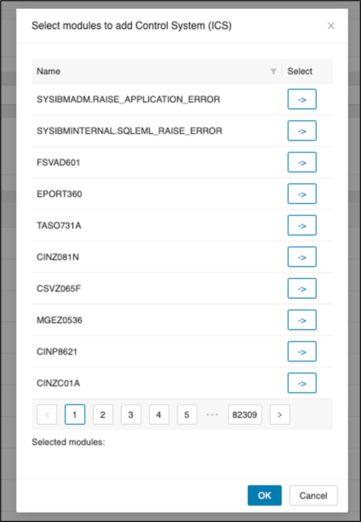
d. Click -> beside any module to select it. Once selected, the module will be grayed out and will appear in the list of selected modules at the bottom of the window.
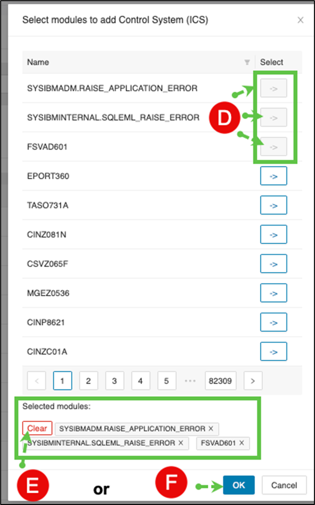
e. If you wish to remove selections, click Clear to remove all chosen modules, or click beside individual modules to remove them from your selection.
Or
f. When satisfied with your selections, click OK to add the selected modules to the taxonomy.
Omitting a Module from a Taxonomy
To omit (temporarily exclude) a module from a taxonomy:
-
Follow steps a and b above to select your taxonomy and display its associated modules.
-
Locate the module you wish to exclude, then toggle the “Omitted” slider next to that module.
This action will remove the module from being displayed in the taxonomy graph, allowing you to control which modules appear in visual representations without permanently deleting them.
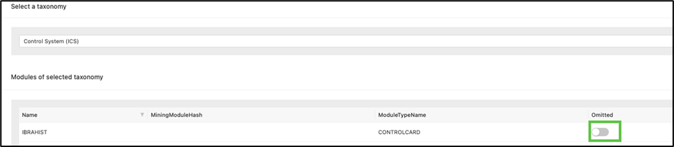
The selected module when then switch to blue symbolizing on.

Removing a Module from a Taxonomy
If a module isn’t needed, you can simply remove it by clicking Remove corresponding to the module.
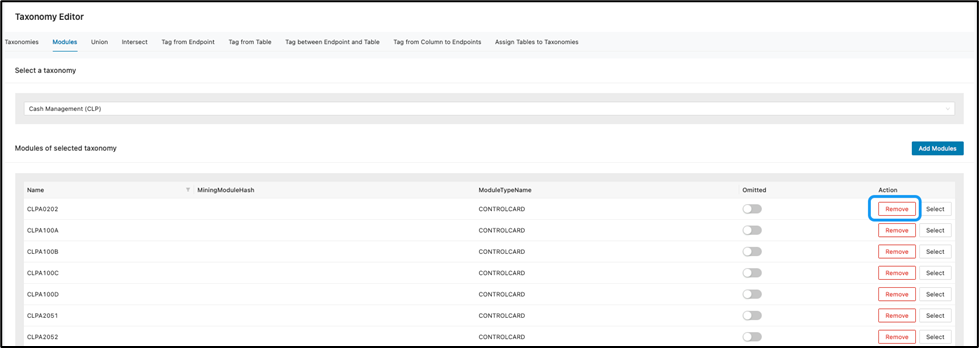
However, the same can be added back by clicking Add Module and search for the deleted item. For instance, CLPA0202 was removed but you decided to add it back.
- Click Add Modules .

The select modules to add to the taxonomy window will display listing modules.
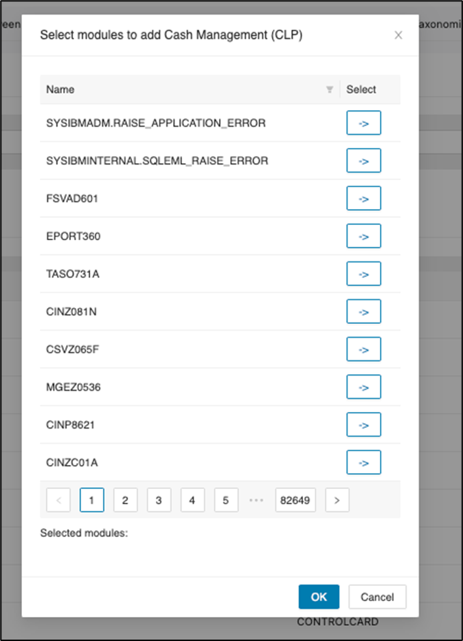
b. Click on the filter icon to limit the search to the deleted module.
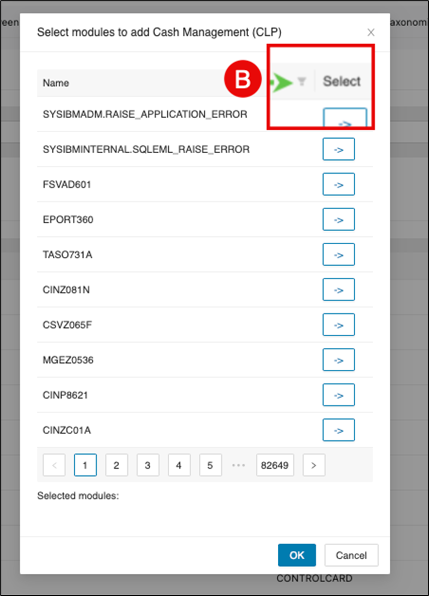
c. Enter the deleted module name in the filter window to search and then click the search icon.
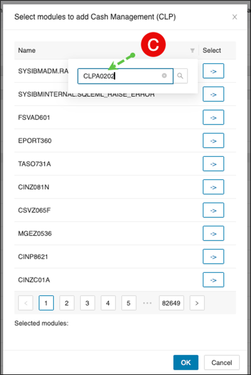
d. The deleted module should then display as below. Click -> to add the module back to the taxonomy.
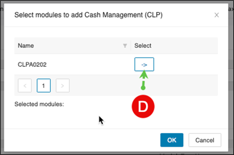
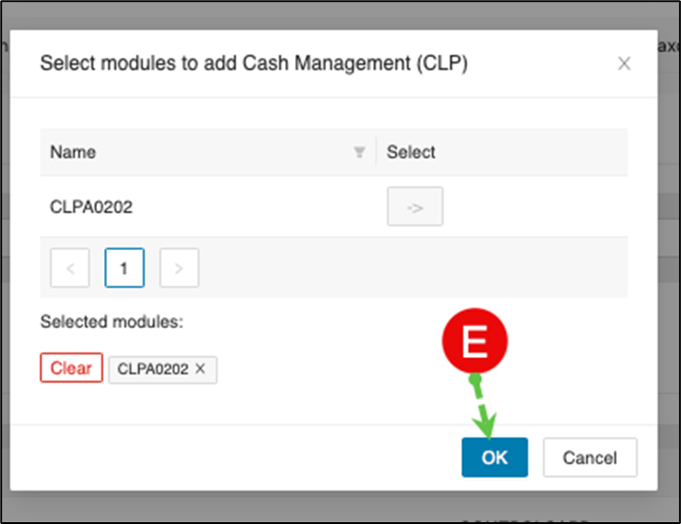
e. After you click ->, the module name appears under the selected modules section. You can clear that module or add more modules before you finish. When you are satisfied, click OK.
Actions on selected Taxonomy
The Modules tab provides a section at the bottom of the page to delete the selected taxonomy or render it.
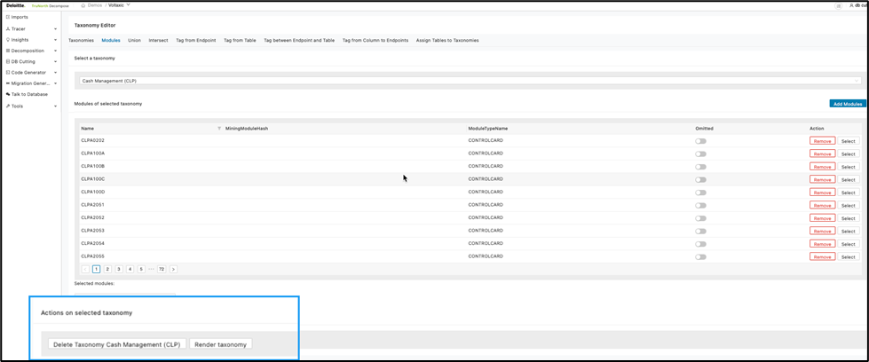
Again, deletion of a taxonomy is irreversible so be mindful before performing this action.
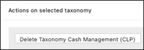
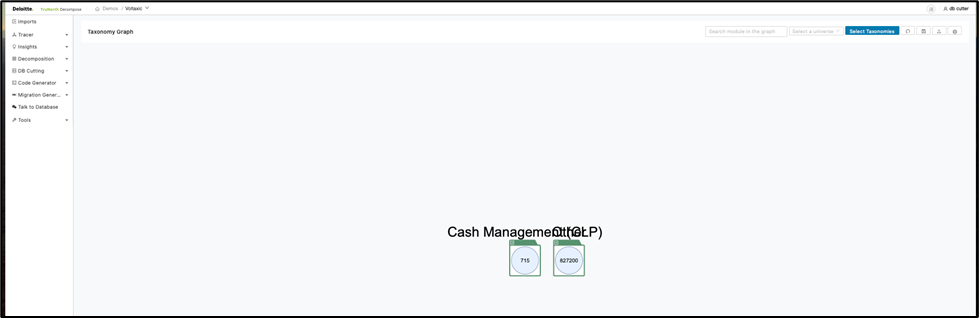
Rendering a taxonomy opens the Taxonomy Graph page and shows the selected taxonomy.
As below:
This completes the Modules tab section.
Union tab
The “Union” function, as the name suggests, is used to generate a taxonomy that is a combination of all existing taxonomies. Essentially, it sums up all the modules present across these taxonomies. The relationship between the modules inside the taxonomy will be copied to the union taxonomy.
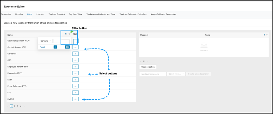
When selecting the Union tab within the Taxonomy Editor, all taxonomies will display on given pages.
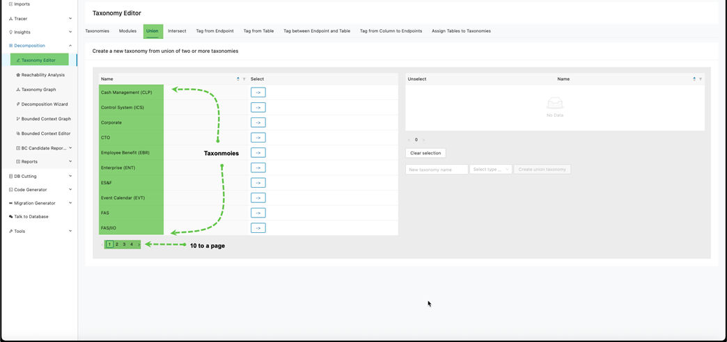
To combine taxonomies that have similar modules you could search for taxonomies to select or click -> corresponding to a taxonomy name.
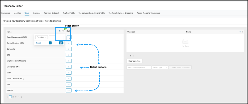
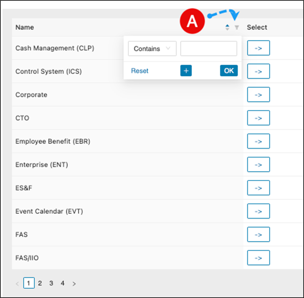
Search for taxonomy using filtering
a. Click on the filter icon.
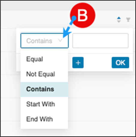
b. Select the preferred “how to filter” mechanism by clicking the drop-down arrow and select an option.
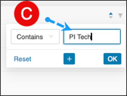
c. Enter the taxonomy name you are searching.
d. Optionally, click the if additional conditions is needed for a refined search of a taxonomy.
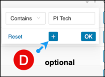
If selected, an additional search field will display as below. If selected, an additional search field will display as below.
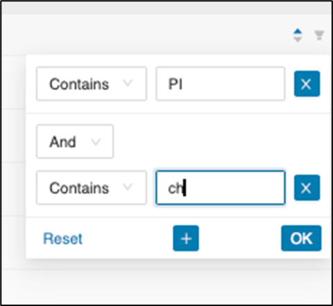
You can add as many conditions as needed.
e. Once satisfied, click on OK .
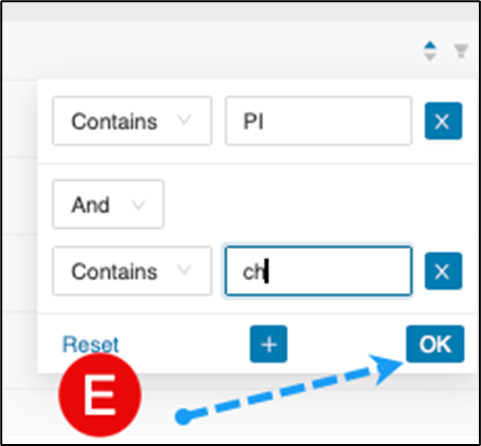
The search will then display the result.
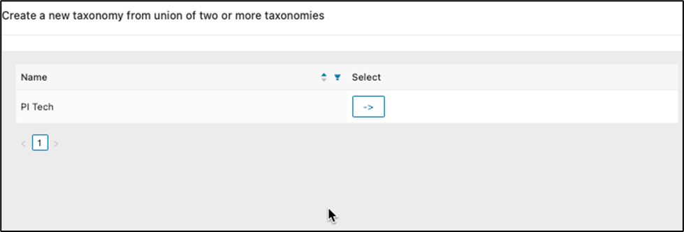
Combining taxonomies to add a union
a. Select the taxonomies from the list of available taxonomies by clicking -> . -> will gray out once a taxonomy has been selected.
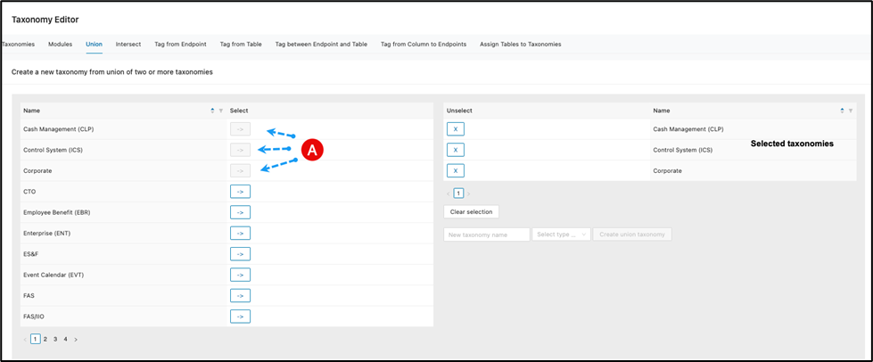
To deselect a taxonomy from the union, click Clear selection or click beside the taxonomy. To clear every taxonomy on the right-hand side, click Clear Selection.
If you are okay with your selections, move to the next step.
b. Enter a new taxonomy name, select the type from the dropdown and then click Create union taxonomy .
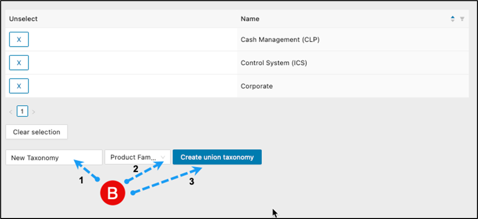
The tool will process and then create a new taxonomy.
c. Search for the new taxonomy to verify the creation.
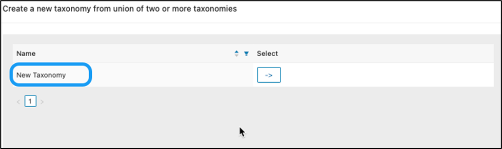
This completes the Union Tab section.
Intersect tab
In this tab, you identify and extract overlapping elements between two or more taxonomies. This is valuable for focus work—such as finding commonalities, redundancies, or shared features—in your data sets or classification schemes.
When selecting the “Intersect” tab within the Taxonomy Editor, all taxonomies will display on given pages.
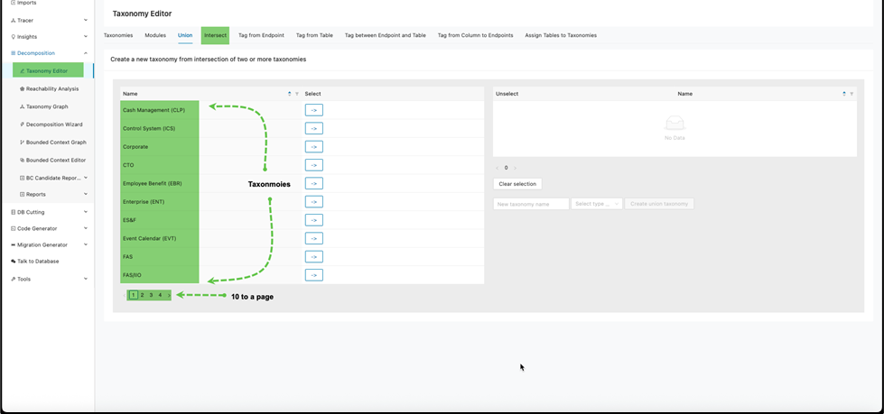
To combine taxonomies that have similar modules you could search for taxonomies to select or click on -> corresponding to a taxonomy name.
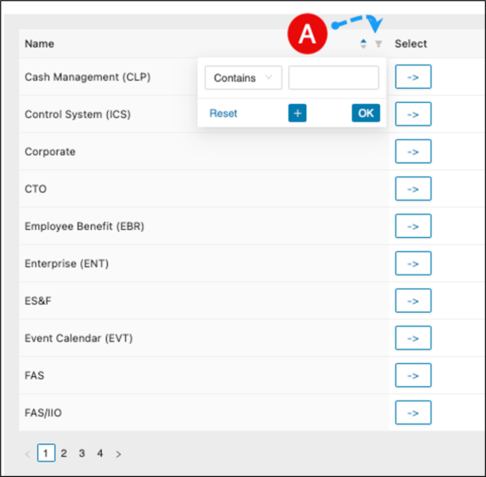
Search for taxonomy using filtering
a. Click on the filter icon.
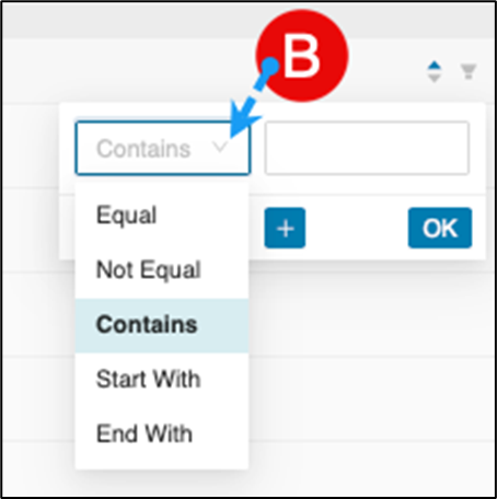
b. Select the preferred “how to filter” mechanism by clicking the drop-down arrow and select an option.
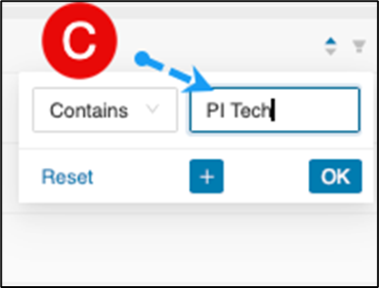
c. Enter the taxonomy name you are searching.
d. Optional, click the if additional conditions is needed for a refined search of a taxonomy.
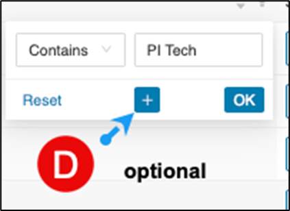
If selected, an additional search field will display as below.
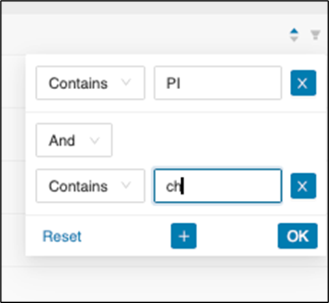
You can add as many conditions as needed.
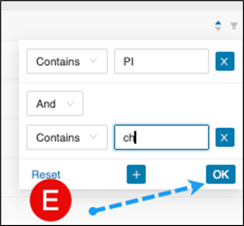
e. Once satisfied, click on OK .
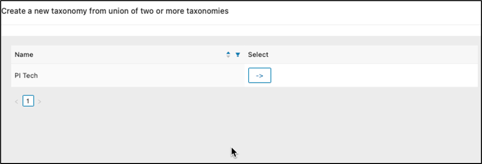
The search will then display the result.
Tag from endpoint tab
Use this feature to create or edit a taxonomy by building a module chain that starts at an endpoint module and follows the endpoint connections until no more connections are possible. This feature determines the module where the chain starts.
When selecting the “Tag from Table” tab, one needs to understand what is being displayed.
-
Incoming relations (the number of incoming relations to other modules)
-
Outgoing relations (the number of outgoing relations to other modules)
-
Read Queries (the number of read queries to databases)
-
Write Queries (the number of write queries to databases)
-
Total number of pages which capsulates the total number of modules as 10 modules displays per page.
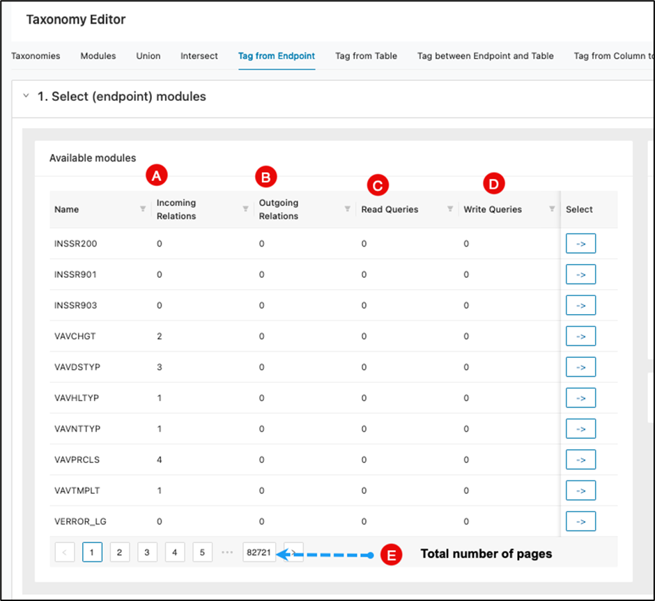
One needs to have a strategy on where to begin when dealing with an extremely high number of modules. You can start small or large so in the following scenario, we will start small to give an idea on how to use “tag from endpoint”.
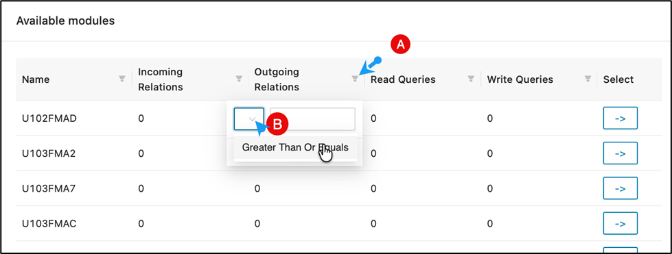
Each column header has filtering which has currently has an option to display “greater than or equals to” to be set for incoming\outgoing relations and read\write queries.
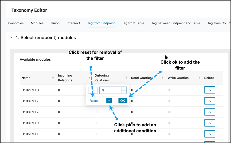
Adjust the filtering for outgoing relations to 5. You can remove the filter by clicking on "Reset" or adding additional conditions by clicking the plus symbol. Once everything looks okay with your filter click OK .
Upon clicking OK , your results should display as below:
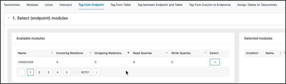
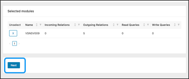
Next, click on -> .

Module VSNSV009 will now appear in the selected modules pane. Click Next to continue.
You will now choose or create a taxonomy. This module is already linked to an existing taxonomy, which you may select, or you can opt to create a new, more specific taxonomy if needed. For demonstration purposes, let’s define a new taxonomy with an easily identifiable name. The name can always be changed later after completing the tagging process.
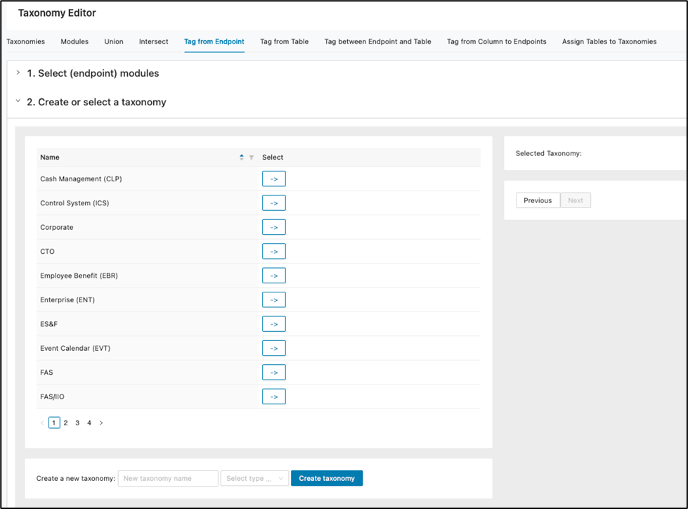
At the bottom of the main windowpane, enter “Tag From Endpoint Taxonomy”, select the “Product Family” type and then click Create taxonomy .

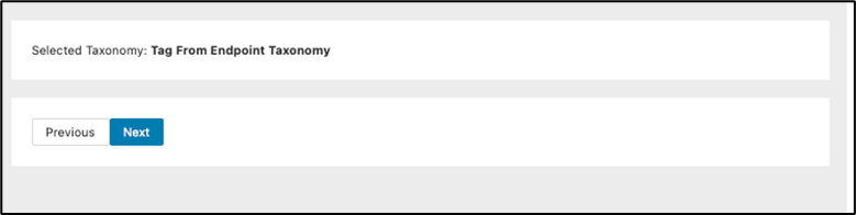
The newly created taxonomy will then show as being selected. Click Next .
The screen will now display the assigned taxonomy and tag all modules being called by the module you selected. Click Assign taxonomy to begin tagging from VSNSV009 to the last chained module.
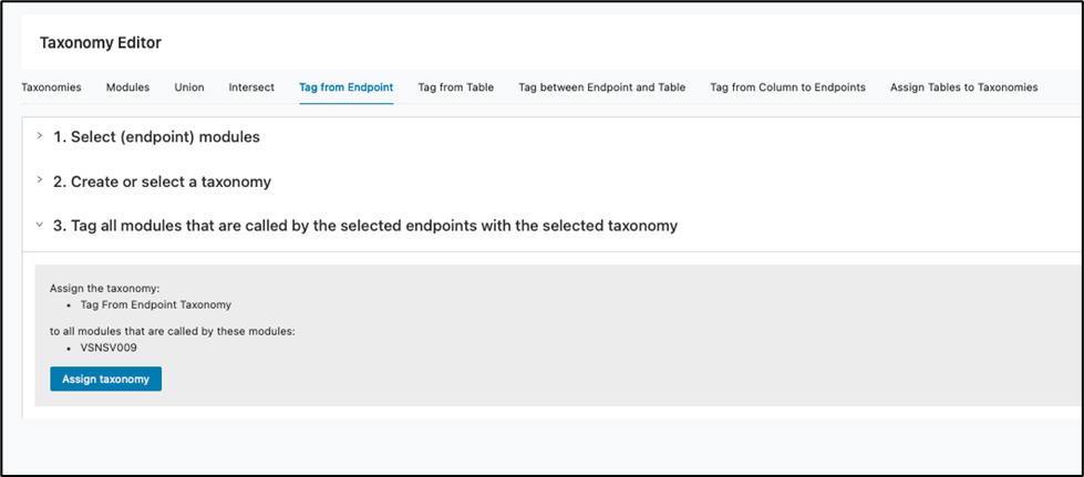
The process will then display a banner message indicating the number of modules tagged.

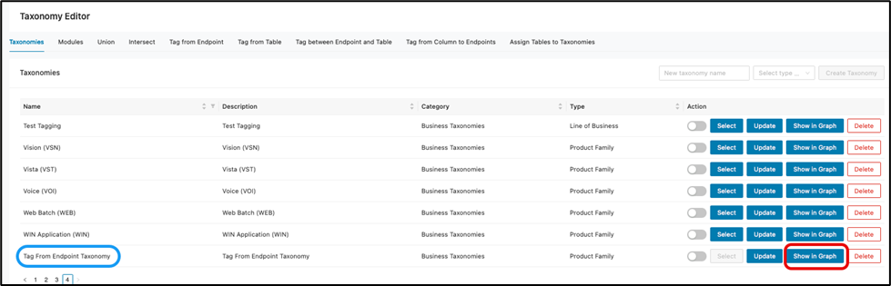
You may then go to the taxonomies tag to select your new taxonomy and then click Show in graph to get a visual display.
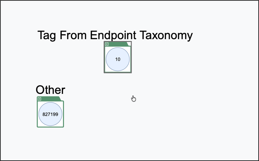
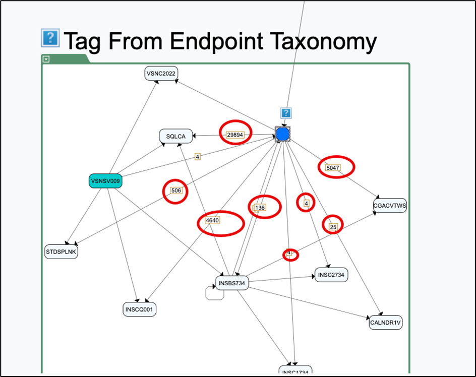
Below, you will see the taxonomy you created displaying 10 modules as specified by the tagging.
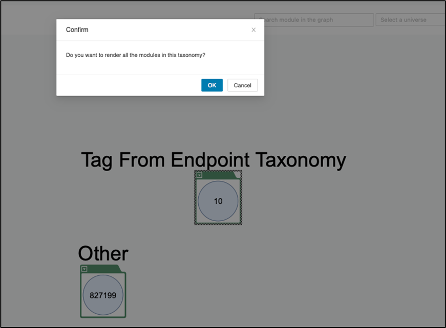
Double-click anywhere on the green bar to render all modules in the taxonomy, then click OK to continue.
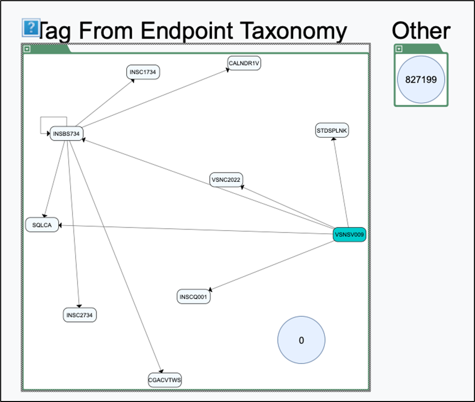
Below, you will see the highlighted module with directional arrows pointing to all related modules, whether they are linked in a chain or have direct connections.
One could even go further to see relations with other taxonomies by showing edges to others.
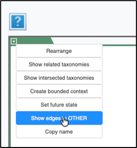
This will then display a bi-directional line to the other taxonomy group.
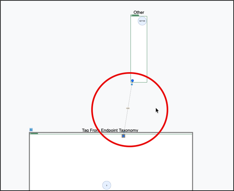
We also see a number on the bi-directional line which indicates the total number of incoming and outgoing connections which tallies to over 47 thousand.
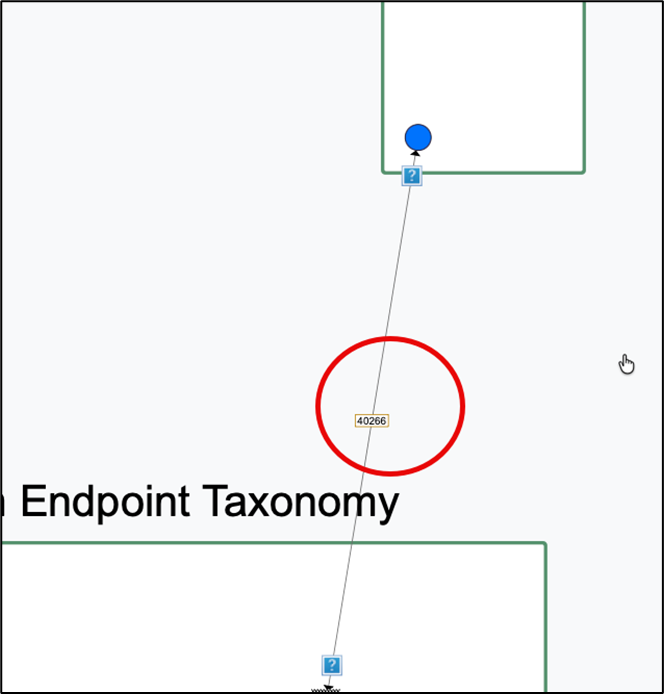
We can explore the connections further by right-clicking on the blue dot within the “Tag from Endpoint Taxonomy”. This will then display two options:
-
Expand outgoing boundary modules
-
Expand incoming boundary modules
When expanding outgoing boundary modules, we see four connections going out from the original “VSNSV009” module selected when initiating tagging.
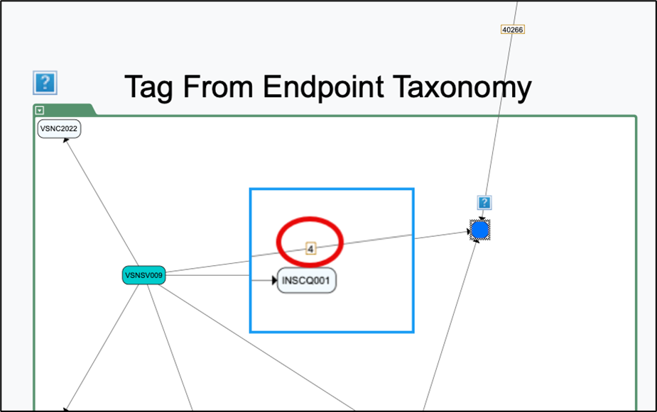
When you expand the incoming connections, you’ll see the total count for each connected module. These connections can be discussed further with the customer, and it may be possible to move the module to a different taxonomy based on the customer’s preferences.
Tag from table
Use this feature to create or edit a taxonomy by building a chain that starts from a module with no incoming relation and ends at a module associated with a table in the module queries file. The chain traverses all modules in between. This feature determines the module where the chain ends.
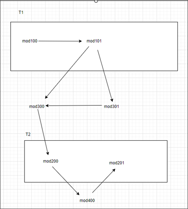
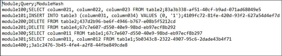
From the module relations and taxonomies modules file, if the above module relationship diagram is considered, as an example and the module queries file is observed as below.
For example, the below chain of modules can be created and assigned to an existing taxonomy or a new taxonomy.
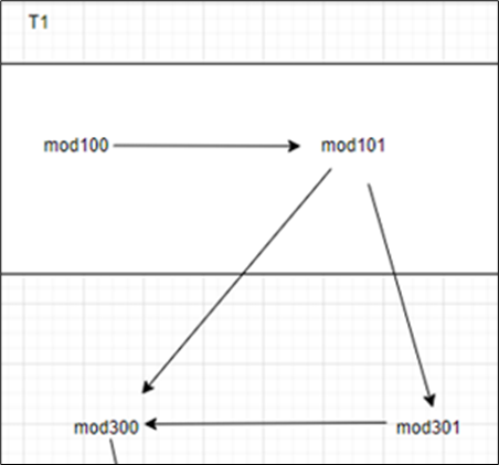
In this case the ending module would be module300 that is associated with table1 from the module queries file. So, in this case it should be tagged from table1.
In the left navigation panel, navigate to Decomposition > Taxonomy Editor and switch to the "Tag from Table" tab.
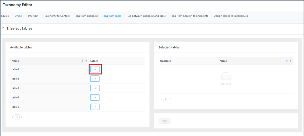
From the Available tables table on the left-hand side, select the tables using the -> .
The tables can be sorted or filtered based on the Name to narrow down your search. If you need to reset the filter, simply click Reset , and it will display all available tables.
Select the tables using the -> alongside the table.
Once the tables move to the Selected tables window, it can be filtered or sorted based on the Name to narrow down your search. If you need to reset the filter, simply click Reset , and it will display all available tables.
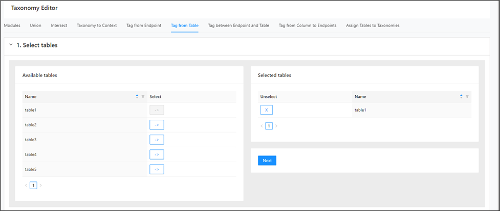
If you wish to deselect any table listed on the right-hand side, click the next to it. It will move from the right side to the left side, indicating that it is deselected.
Then, click Next .
Or create a new taxonomy by entering a name, selecting a type.
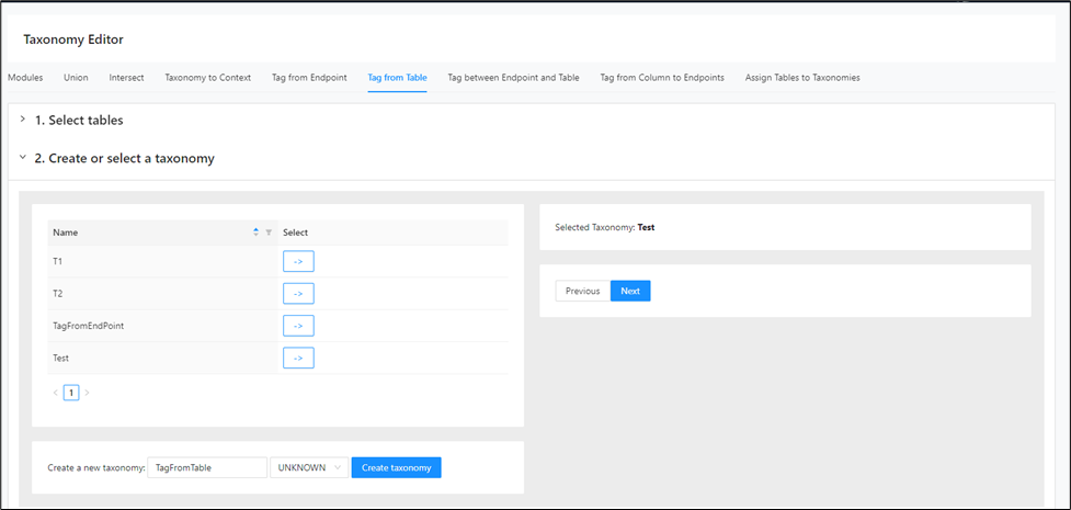
And then click Create taxonomy .
Once the taxonomy is selected (either new or an existing), it will appear on the right-side window.
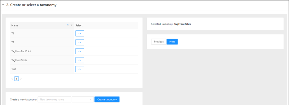
Click Next .
A message appears indicating the module assignment.
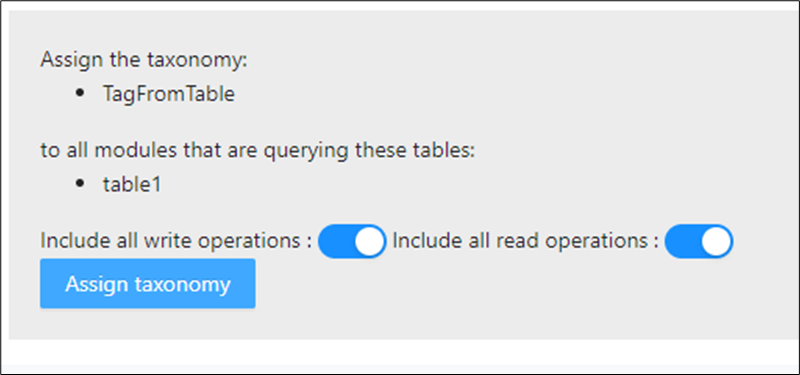
Here either the read (SELECT) queries or Write (INSERT, UPDATE, DELETE) queries associated with the table can be selected or both.
Finally click on Assign Taxonomy .
After the assignment, a message appears indicating how many modules are assigned to the taxonomy.
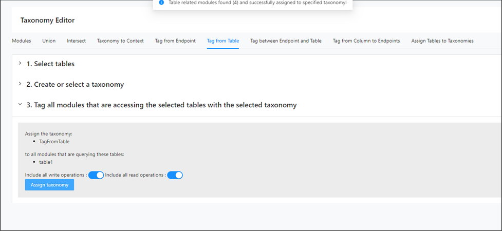
You can verify the assignment from the Taxonomy Graph.
Tag between endpoint and table
Use this feature to create or edit a taxonomy by building a chain that starts from an endpoint module and ends at a module associated with a table in the module queries file. The chain traverses all modules in between. This feature determines both the start and end modules.
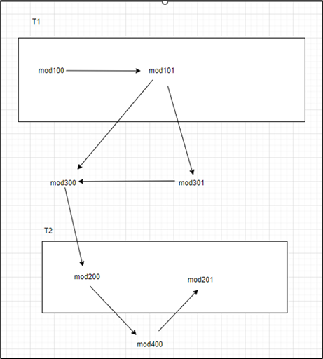
From the module relations and taxonomies modules file, if the above module relationship diagram is considered, as an example and the module queries file is observed as below.
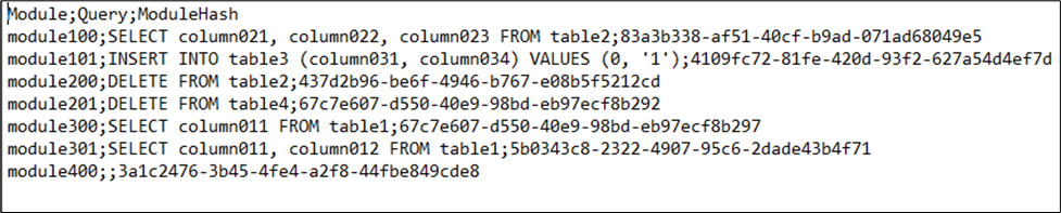
For example, the below chain of modules can be created and assigned to an existing taxonomy or a new taxonomy.
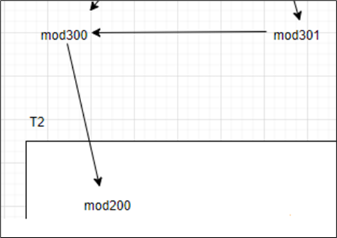
In this case the starting module would be mod301 (endpoint module) and ending module would be module200 that is associated with table2 (DELETE query) from the module queries file. So, in this case it Should be tagged from table1 with Only Write Query.
Should be tagged from table1 with Only Write Query.
In the left navigation panel, navigate to Decomposition > Taxonomy Editor and switch to the "Tag between Endpoint and Table" tab.
From the Available modules table in the left-hand side, select the modules using the -> .
The modules can be filtered based on the Name, Incoming Relations, Outgoing Relations, Read Queries and Write Queries to narrow down your search. If you need to reset the filter, simply click Reset , and it will display all available modules.
Select the modules using the -> alongside the module.
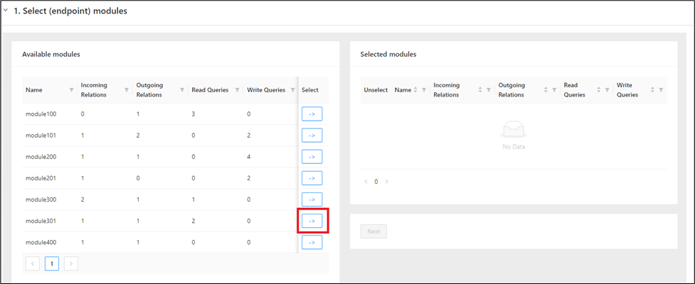
Once the modules move to the Selected Modules window, it can be filtered based on the Name, Incoming Relations, Outgoing Relations, Read Queries and Write Queries to narrow down your search. If you need to reset the filter, simply click Reset , and it will display all available modules.
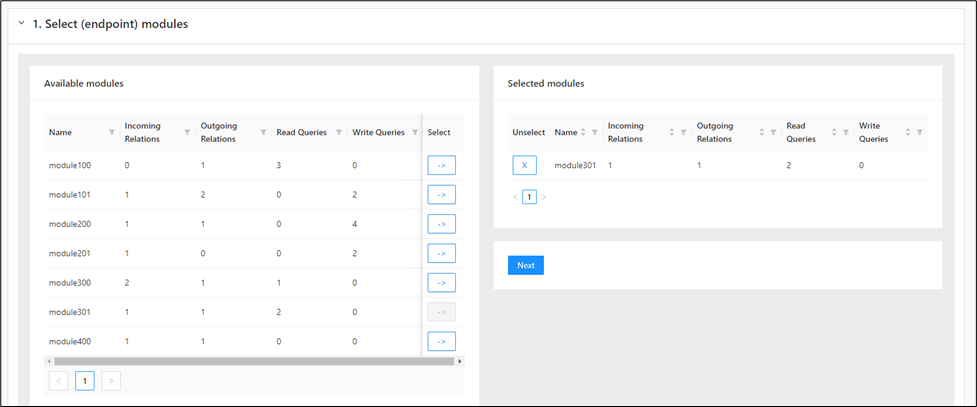
If you wish to deselect any module listed on the right-hand side, click the next to it. It will move from the right side to the left side, indicating that it is deselected.
Then, click Next .
From the Available tables table in the left-hand side, select the tables using -> .
The tables can be sorted or filtered based on the Name to narrow down your search. If you need to reset the filter, simply click Reset , and it will display all available tables.
Select the tables using the -> alongside the table.
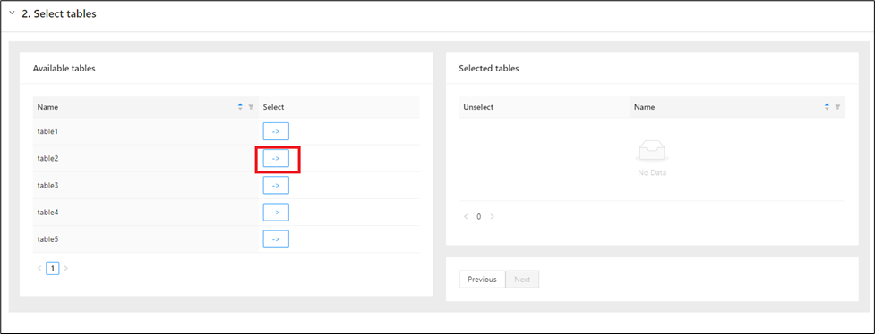
Once the tables move to the Selected tables window, it can be filtered or sorted based on the Name to narrow down your search. If you need to reset the filter, simply click Reset , and it will display all available tables.
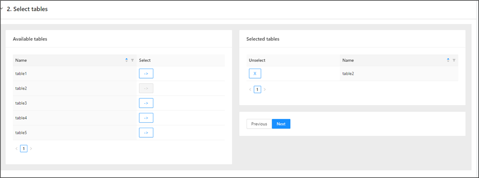
If you wish to deselect any table listed on the right-hand side, click the next to it. It will move from the right side to the left side, indicating that it is deselected.
Then, click Next .
From the taxonomy table, select either an existing taxonomy clicking -> .
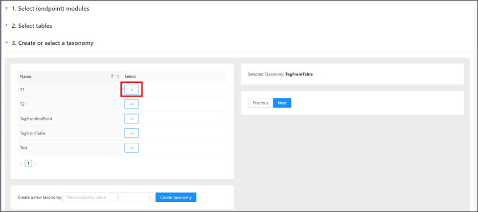
Or create a new taxonomy by entering a name, selecting a type.
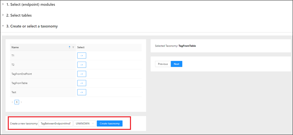
And then click Create taxonomy .
Once the taxonomy is selected (either new or an existing), it will appear on the right-side window.
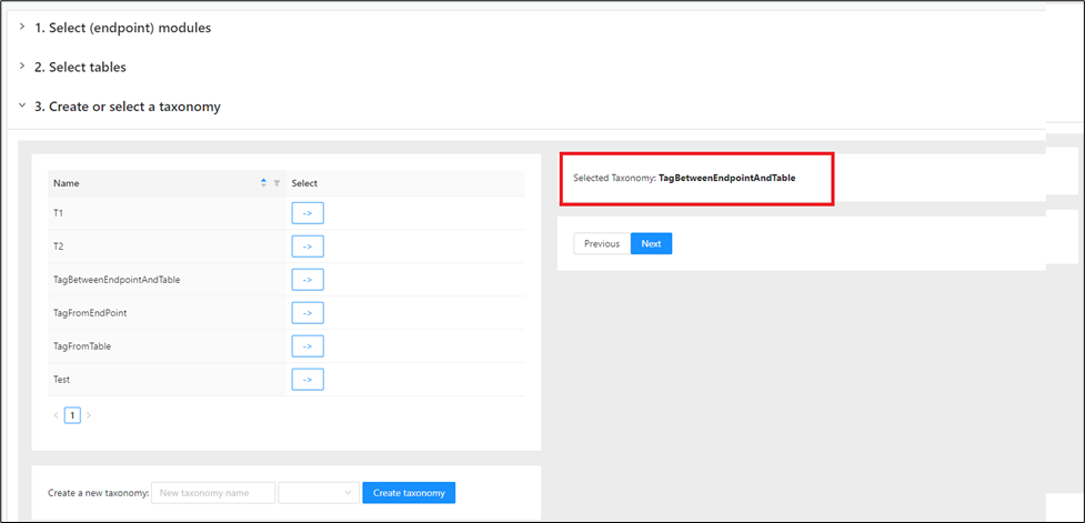
Then, click Create taxonomy .
A message appears indicating the module assignment.
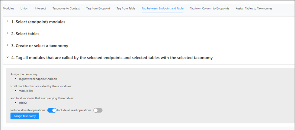
Here either the read (SELECT) queries or Write (INSERT, UPDATE, DELETE) queries associated with the table can be selected or both.
Finally click Assign Taxonomy .
After the assignment, a message appears indicating how many modules are assigned to the taxonomy.
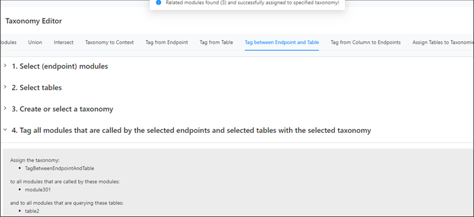
You can verify the assignment in Taxonomy Graph.
Tag from column to endpoints
Use this feature to create or edit a taxonomy by building a chain that starts from an endpoint module and ends at a module associated with a column in a table in the module queries file. The chain traverses all modules in between. This is a more detailed approach than Tag between endpoint and table because it considers columns in the query.
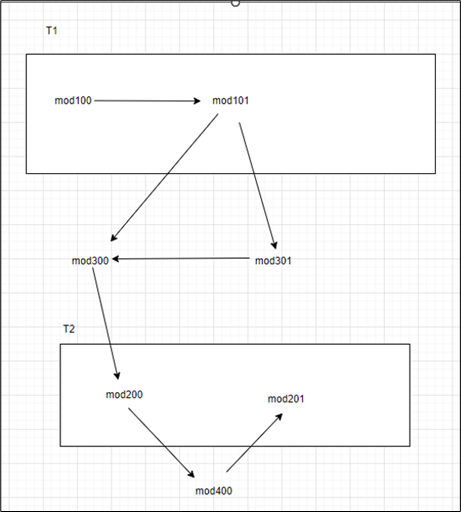
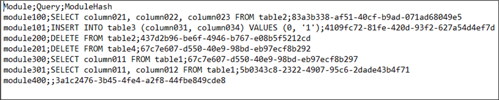
From the module relations and taxonomies modules file, if the above module relationship diagram is considered, as an example and the module queries file is observed as below.
For example, the below chain of modules can be created and assigned to an existing taxonomy or a new taxonomy.
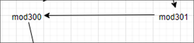
In this case the starting module would be mod301 (endpoint module) and ending module would be module300 that is associated with column011 in table1 as per the module queries file. So, in this case it should be tagged from column011.
In the left navigation panel, navigate to Decomposition > Taxonomy Editor and switch to the "Tag from Column to Endpoints" tab.
From the Select Columns in the left-hand side window, expand schema using , expand the table and then select the column using the -> .
The schema, tables and columns can be sorted or filtered based on the Name to narrow down your search. If you need to reset the filter, simply click Reset , and it will display all available schema, tables, and columns.
Select the column using the -> alongside the column.
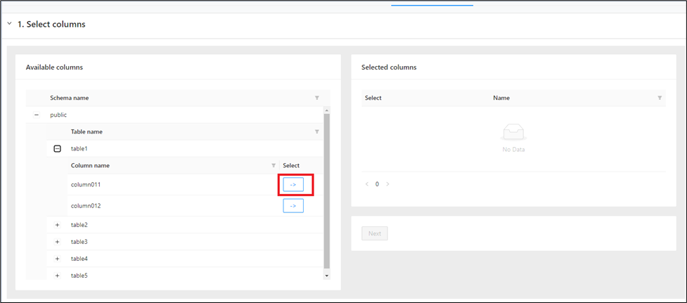
Once the columns move to the Selected columns window, it can be filtered based on the Name to narrow down your search. If you need to reset the filter, simply click Reset , and it will display all available columns.
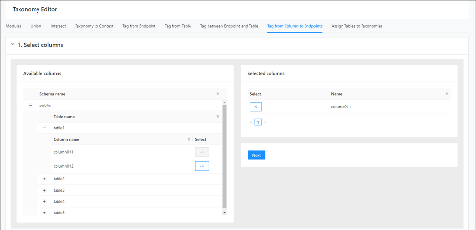
If you wish to deselect any column listed on the right-hand side, click the next to it. It will move from the right side to the left side, indicating that it is deselected.
Then, click Next .
From the Available modules table in the left hand side, select the modules clicking -> .
The modules can be filtered based on the Name, Incoming Relations, Outgoing Relations, Read Queries and Write Queries to narrow down your search. If you need to reset the filter, simply click Reset , and it will display all available modules.
Select the modules using the -> alongside the module.
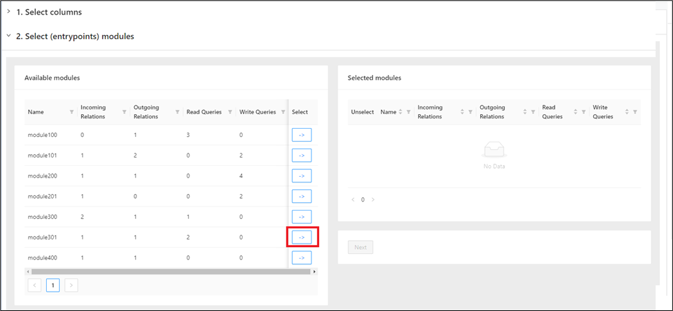
Once the modules move to the Selected Modules window, it can be filtered based on the Name, Incoming Relations, Outgoing Relations, Read Queries and Write Queries to narrow down your search. If you need to reset the filter, simply click Reset , and it will display all available modules.
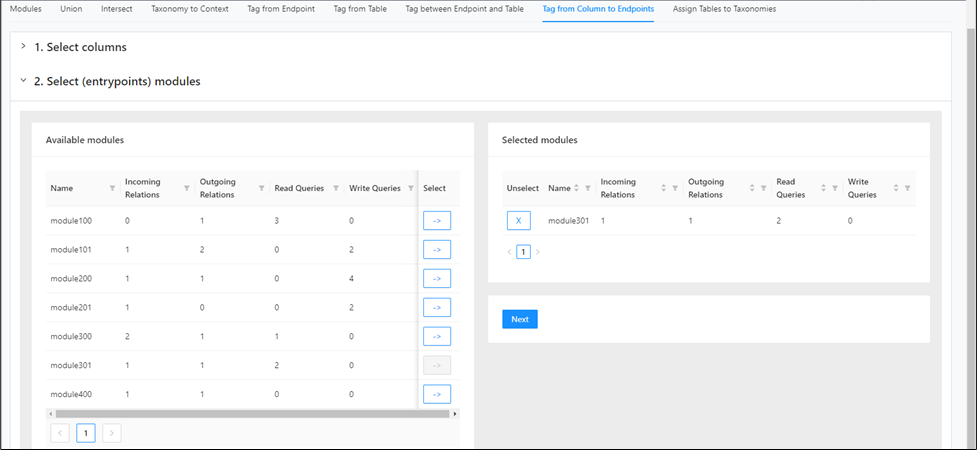
If you wish to deselect any module listed on the right-hand side, click the next to it. It will move from the right side to the left side, indicating that it is deselected.
Then, click Next .
From the taxonomy table, select either an existing taxonomy clicking the -> .
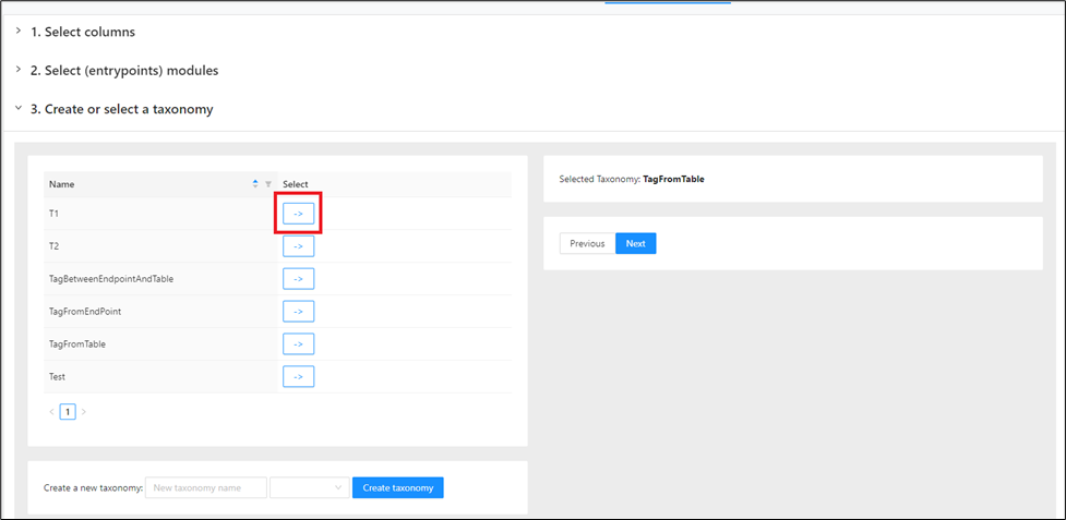
Or create a new taxonomy by entering a name, selecting a type.
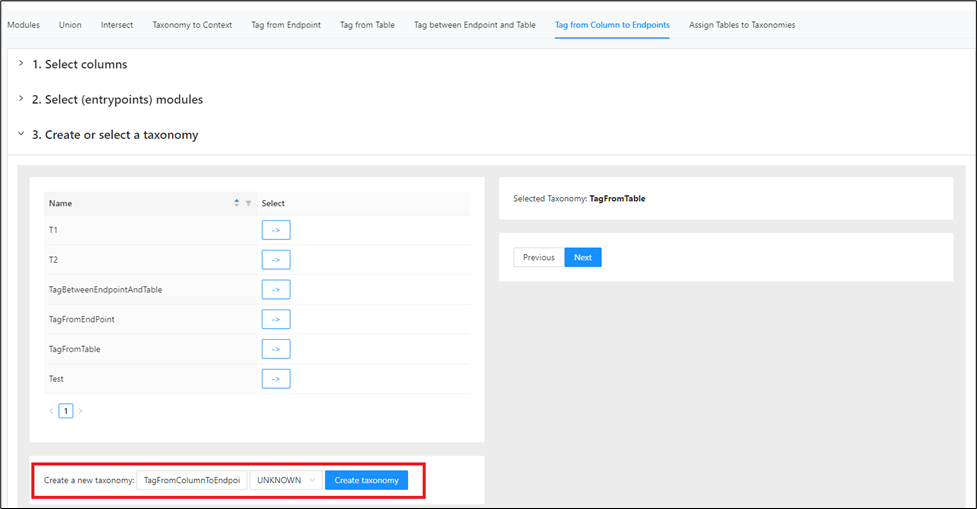
And then click Create taxonomy .
Once the taxonomy is selected (either new or an existing), it will appear on the right-side window.
Click Next .
A message appears indicating the module assignment.
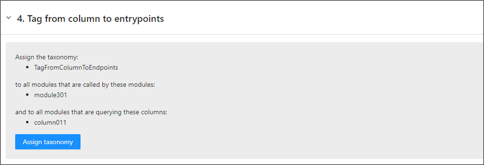
Finally click Assign Taxonomy .
After the assignment, a message appears indicating how many modules are assigned to the taxonomy.
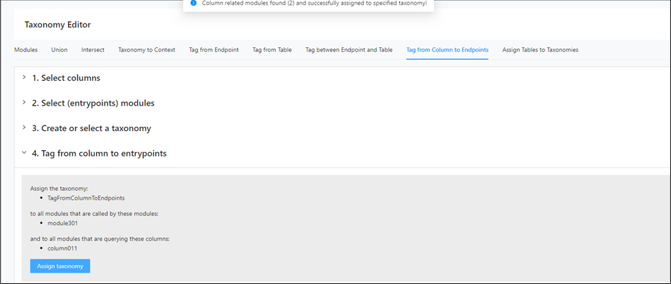
You can verify the assignment in Taxonomy Graph.
Assign table to taxonomies
Use this feature to assign tables to taxonomies instead of modules. It is useful when table ownership is a better starting point than module grouping for the taxonomy you want to build. Use this workflow to connect database objects directly to a taxonomy before moving into later graph and bounded context steps.
In the left navigation panel, navigate to Decomposition > Taxonomy Editor and switch to the "Assign Tables to Taxonomies" tab.
From the Available tables table in the left-hand side, select the tables using the -> .
The tables can be sorted or filtered based on the Name to narrow down your search. If you need to reset the filter, simply click Reset , and it will display all available tables.
Select the tables using the -> alongside the table.
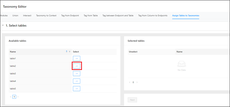
Once the tables move to the Selected tables window, it can be filtered or sorted based on the Name to narrow down your search. If you need to reset the filter, simply click Reset , and it will display all available tables.
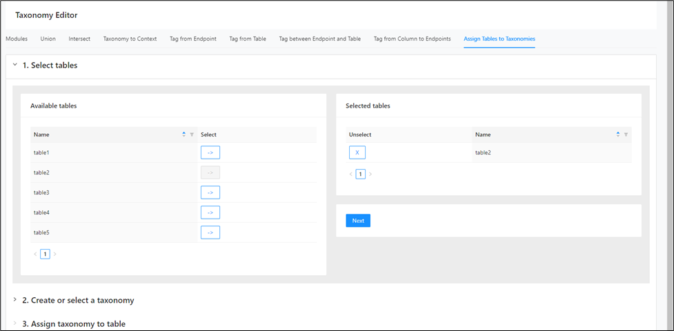
If you wish to deselect any table listed on the right-hand side, click the next to it. It will move from the right side to the left side, indicating that it is deselected.
Then, click Next .
From the taxonomy table, select either an existing taxonomy clicking the -> .
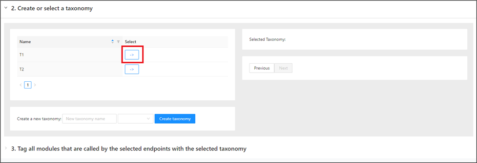
Or create a new taxonomy by entering a name, selecting a type.
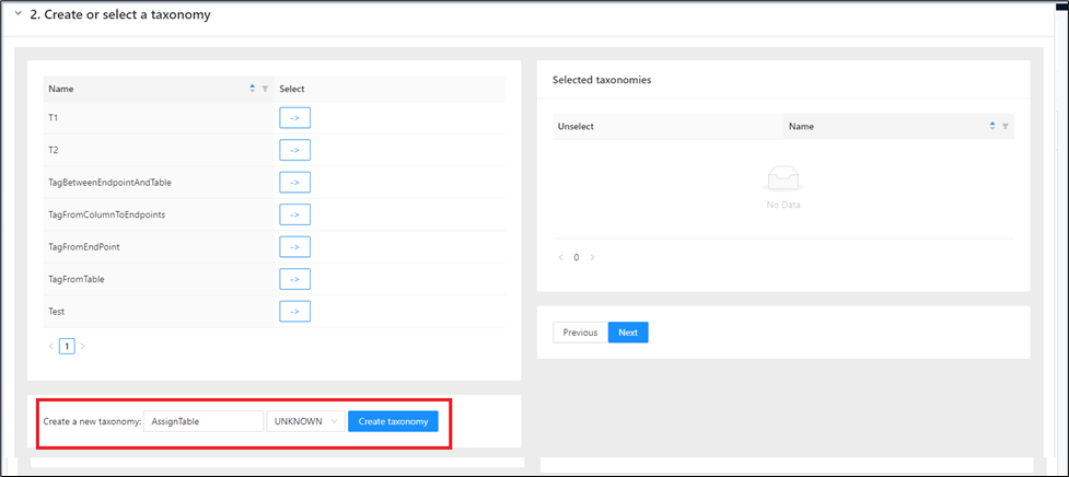
And then click Create taxonomy .
Once the taxonomy is selected (either new or an existing), it will appear on the right-side window.
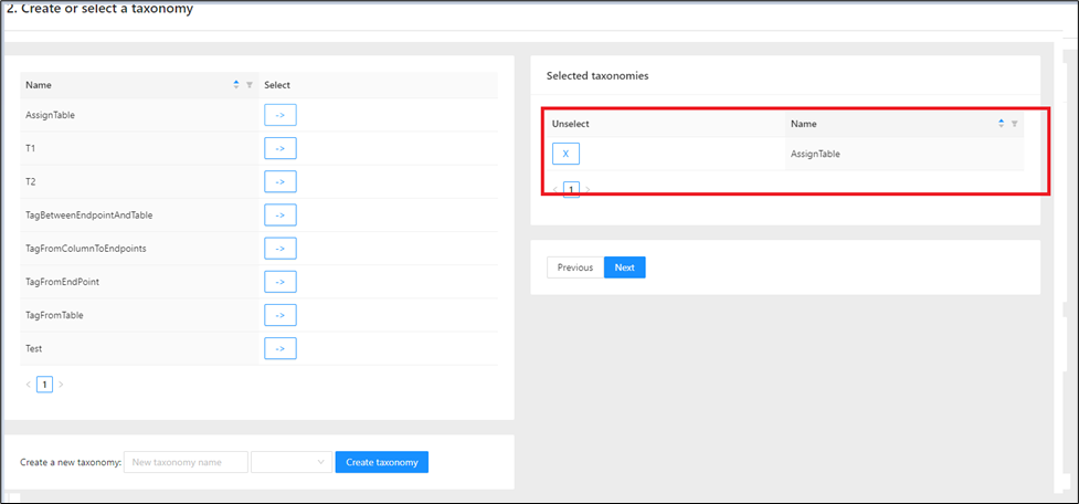
If you wish to deselect any taxonomy listed on the right-hand side, click the next to it. It will move from the right side to the left side, indicating that it is deselected.
Then, click Next .
A message appears indicating the table assignment.
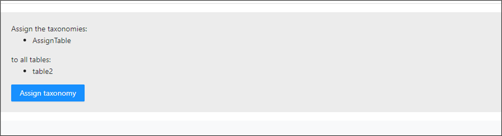
Finally click on Assign taxonomy .
Reachability analysis
Reachability analysis identifies modules in the call chain between an upper boundary taxonomy and a lower boundary taxonomy. It is useful when you want to discover all modules involved between a known entry point and a known downstream boundary. Use this feature to generate taxonomies from actual call-chain structure instead of manual grouping alone.
For example, consider the module relation diagram below.
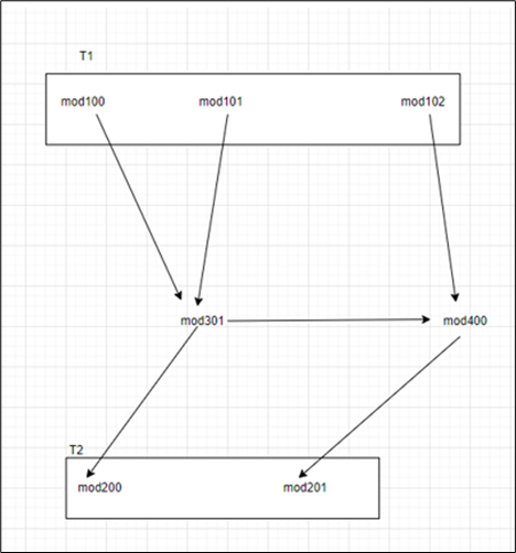
T1 is the upper boundary, and T2 is the lower boundary.
There are three paths from T2 to T1: through mod100, mod101, and mod102.
Reachability analysis creates taxonomies for all modules in the call chain that access these three paths. Additionally, it finds all other modules by walking the call chain downward from the entry points (top-down).
In the left navigation panel, navigate to Decomposition > Reachability Analysis.
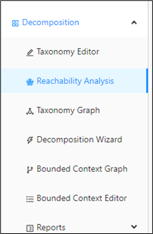
Clear the option shown in the page before you select the upper and lower boundaries.
Select T1 as the upper boundary and T2 as the lower boundary.
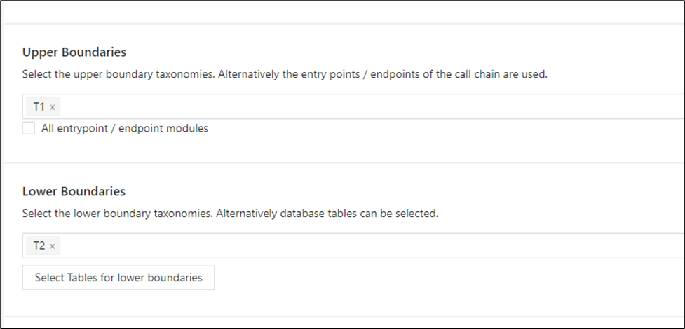
Then click Start Reachability Analysis.
The analysis starts and displays the output after a few seconds.
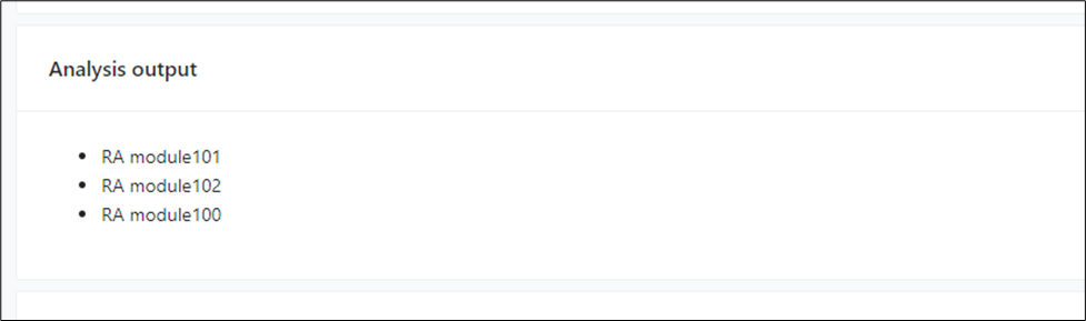
The output creates the taxonomies shown above, containing modules in the call chain.
You can also view the same result visually in Taxonomy Graph by clicking Show in Taxonomy Graph.
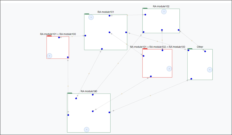
Taxonomy Graph
Taxonomy Graph visualizes taxonomies created in the Mining UI or edited in Taxonomy Editor by using Union, Intersect, Tag from Endpoint, and related options. It also shows the taxonomies created after Reachability analysis. Use this page to analyze taxonomies visually, compare their relationships, and continue editing them as needed.
In the left navigation panel, navigate to Decomposition > Taxonomy Graph.
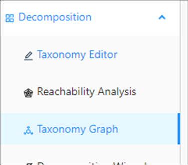
You can also open it directly after Reachability Analysis.
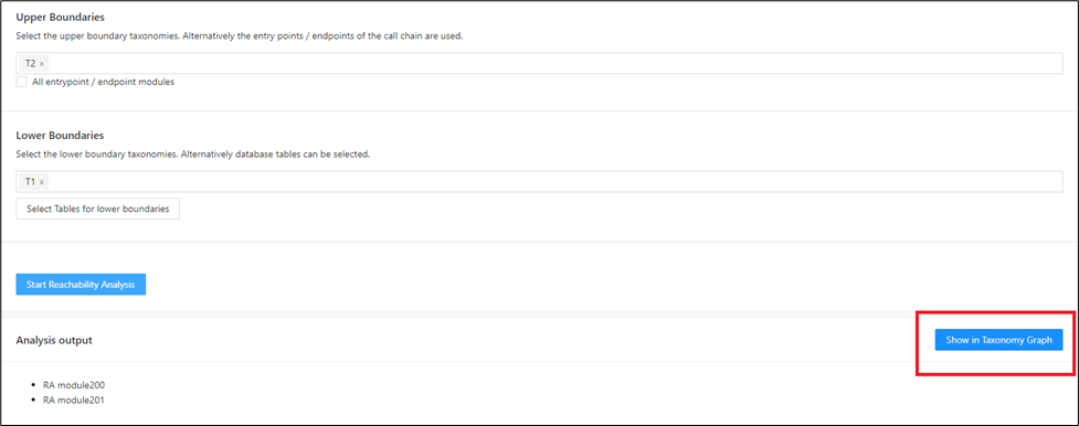
You can also open it from the Modules tab in Taxonomy Editor.
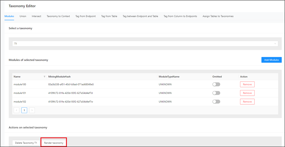
Right-click a taxonomy and select Taxonomies > Show edges to other to display edges to other taxonomies. By default, those edges are hidden.
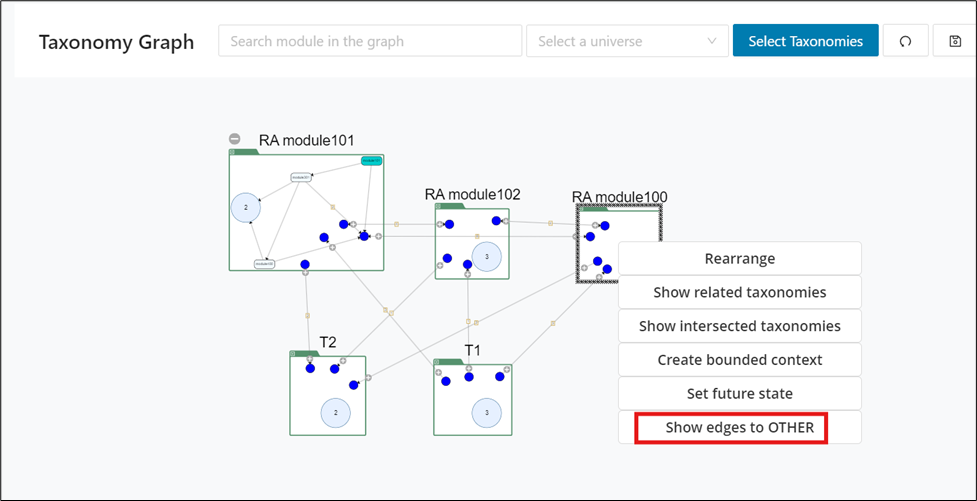
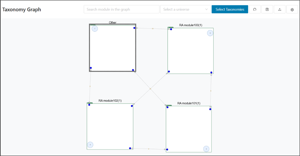
The taxonomies without any edges to Others will display a warning message.
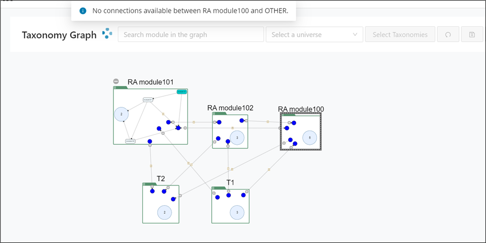
The sections below describe the main Taxonomy Graph features.
Main features
The main feature set is designed to help you control what appears in the graph and how much detail is visible at a given time. These controls are essential when you move from a simple overview to a more focused inspection of taxonomy relationships. Review them first so you can navigate larger taxonomy sets efficiently.
Search taxonomies by module
This will highlight the taxonomies in which the searched module is present by a dark border.
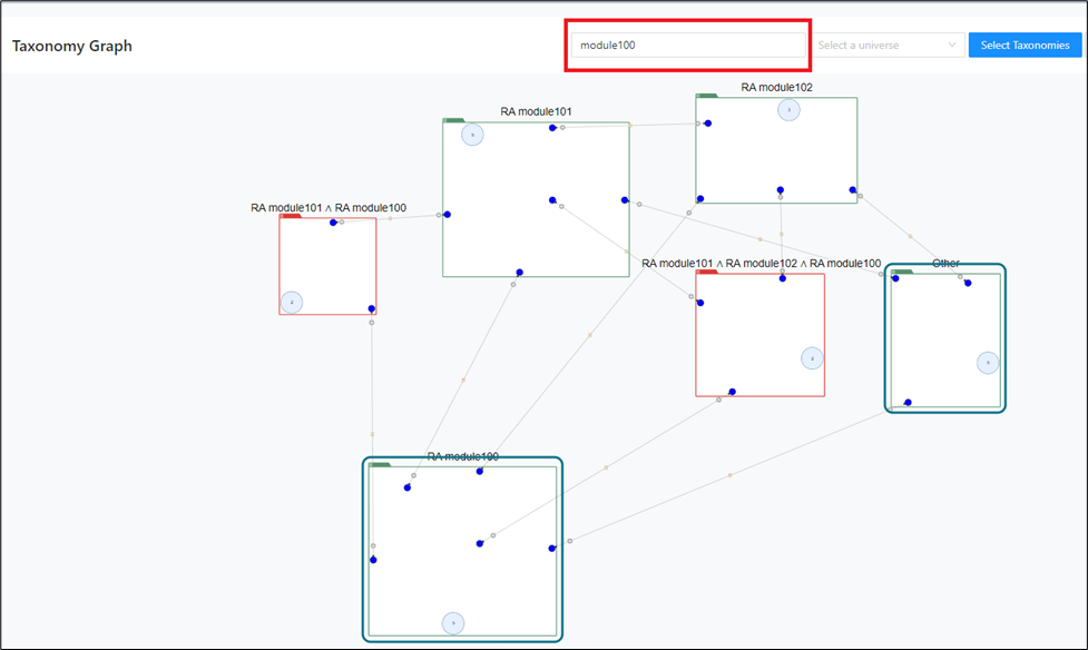
Select a universe
This will compare the taxonomy displayed on the screen to the universe selected. If no universe is selected, the entire set of taxonomies for the project are taken into consideration.
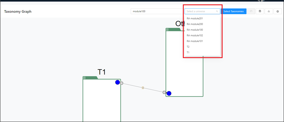
Select taxonomies to display
This will display only the taxonomies that are selected and hide the remaining unselected taxonomies from the graph.
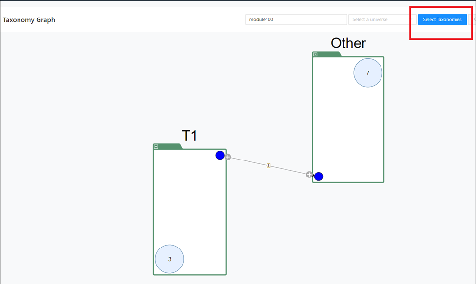
The taxonomies can be selected one by one by clicking on the check boxes alongside them or selected all at once using the checkbox beside Name.
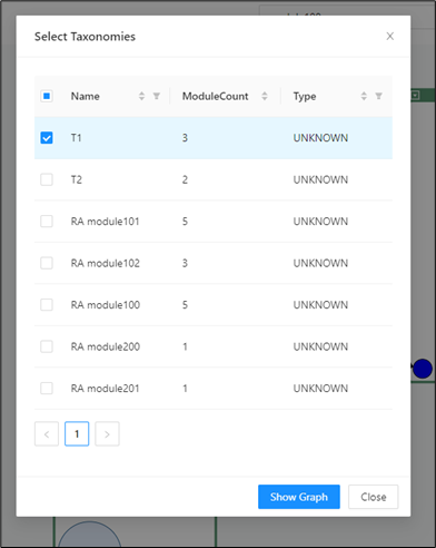
Filters and sorters can be applied here based on the Name, Module Count and Type of the taxonomies to narrow down the results in case of large number of taxonomies.
Save graph configuration
Use this option to save the current graph state with the module counts. This is useful if you later edit taxonomies and want to reload the saved state.
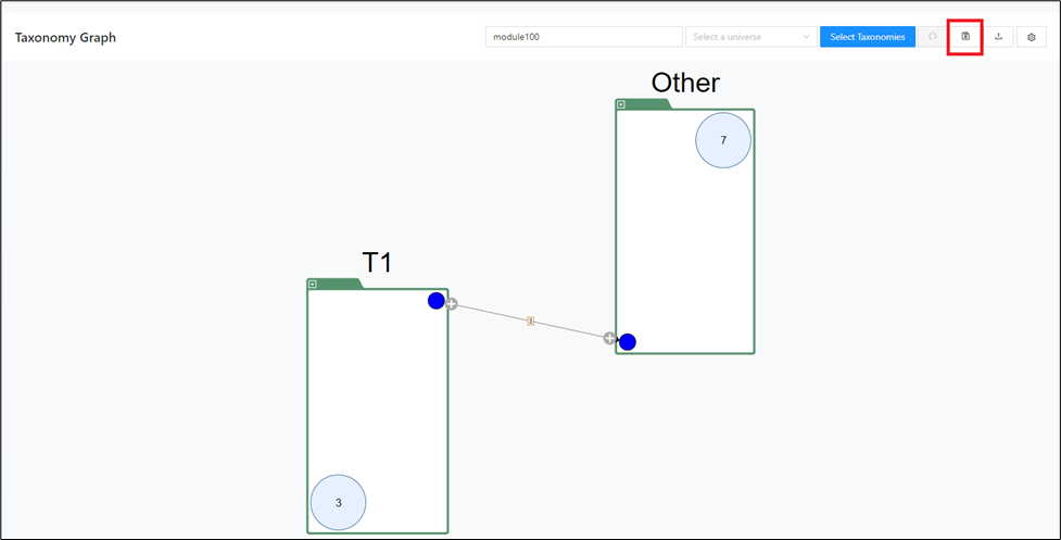
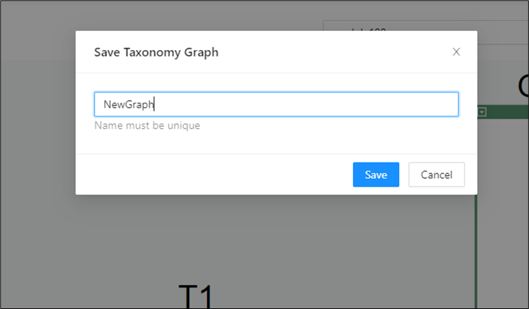
A name needs to be provided and saved.
Load a saved graph
Use this option to load a graph that you saved earlier. It restores the taxonomy state, especially the modules present in each taxonomy, if later changes need to be rolled back.
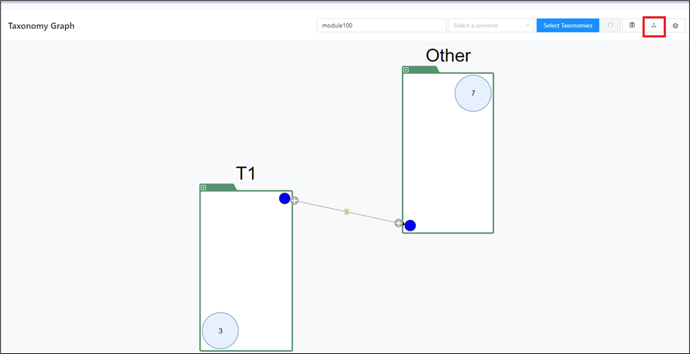
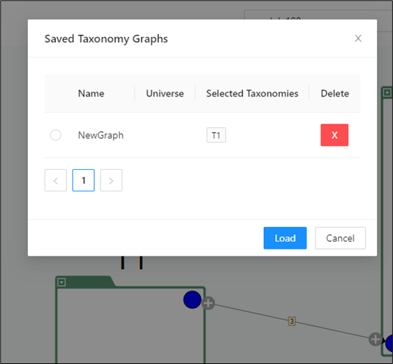
The configuration needs to be selected and loaded.
Graph options
Use this menu to export the graph as SVG, GraphML, or PDF, or to download the taxonomy report and taxonomy module report.
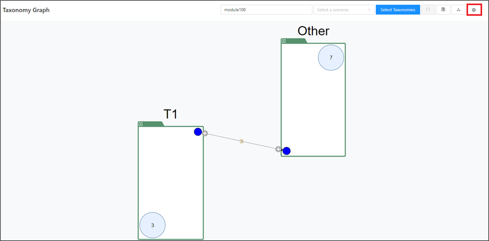
Clicking on the options below does the action mentioned earlier.
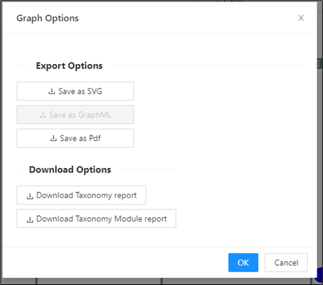
Undo
The undo icon is used to revert any move operations (moving modules to and from taxonomies).
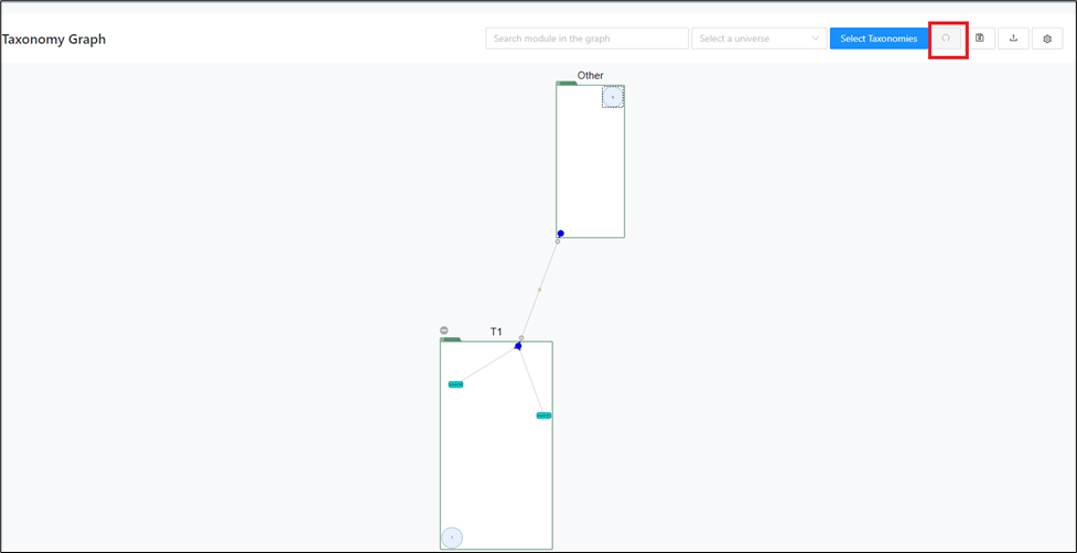
Explanation of the graph elements
The graph uses several visual elements to show taxonomy structure, shared resources, and module-level relationships. Understanding these elements makes the later editing actions easier to interpret and less error-prone. Use this section as a quick legend before you expand nodes or move modules.
The graph shows:
Taxonomy names
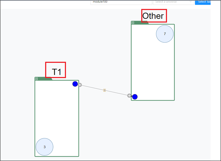
Boundary modules
Boundary modules are modules that create an external connection to another taxonomy.
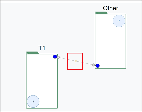
Drawer window
The number on the edge connecting the two taxonomies shows the number of external connections between the two taxonomies.
Clicking an edge opens a drawer that shows the boundary modules or all modules in the connected taxonomies. You can move modules from one taxonomy to the other from this drawer.
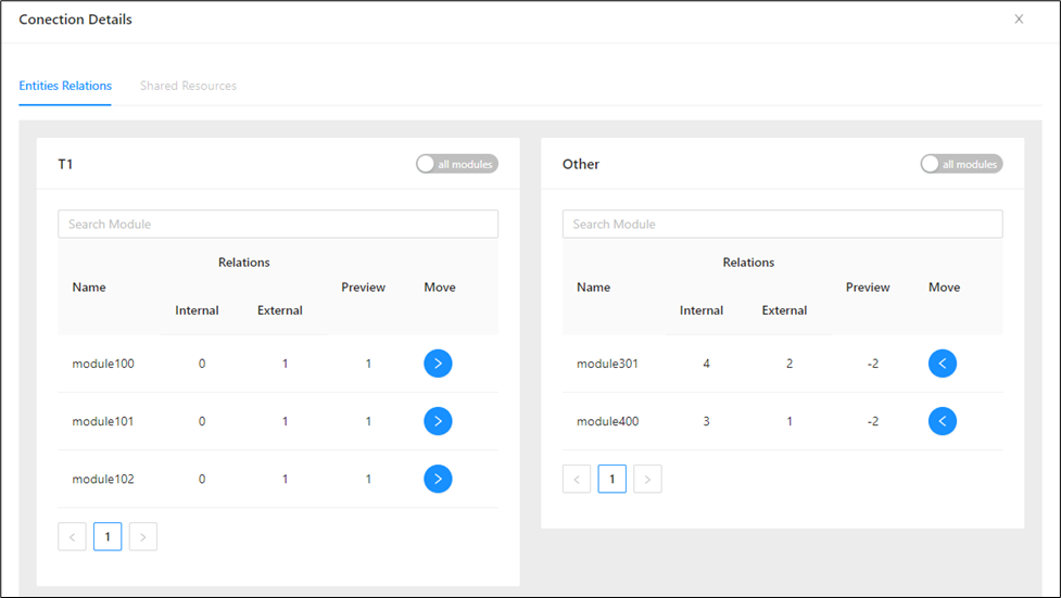
This drawer shows the names of the boundary modules for both the taxonomies along with number of internal, external connections and preview. This is the number of connections affected if the module is moved to the other taxonomy.
Use the search bar to find a module.
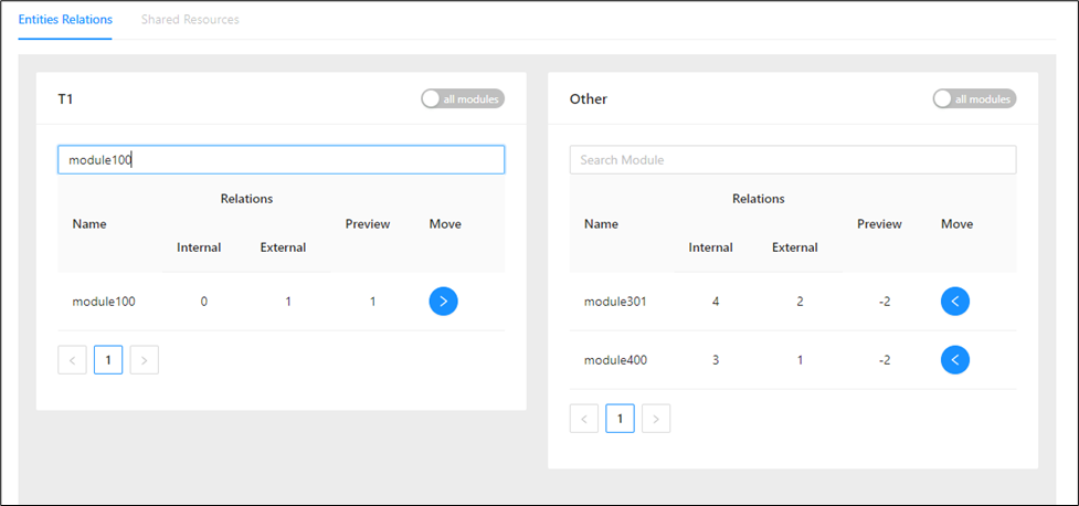
Modules can be moved from one side to the other (left side taxonomy to the right-side taxonomy or vice versa) by either or .
To see all modules, click on the all modules toggle:
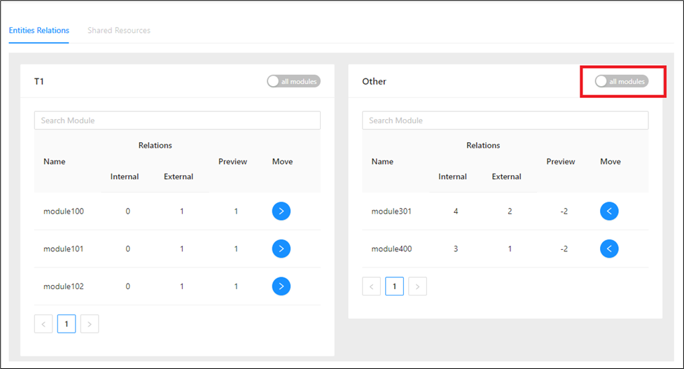
To see only boundary modules, click on the boundary modules toggle:
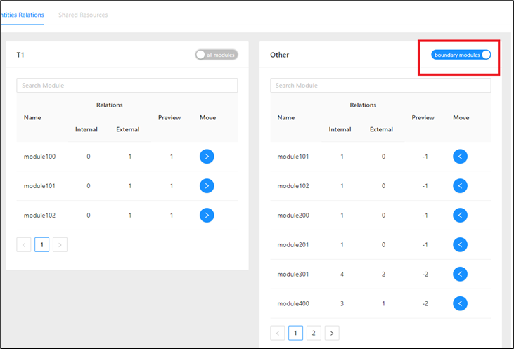
If the all modules switch is not possible to be clicked it means boundary modules = all modules.
Shared resource
This contains tables/files that are used by modules from at least two taxonomies on the graph. Both taxonomies have an edge to the resource intersection.
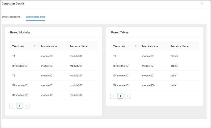
Unexpanded modules
The unexpanded modules are shown in the module circles inside the taxonomy.
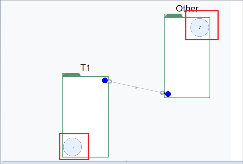
Expand taxonomies
Taxonomies can be expanded to see the relations between the modules inside the taxonomies (internal connections) and to other taxonomies (external connections)
You can do this at once by clicking the expand icon on the edge.
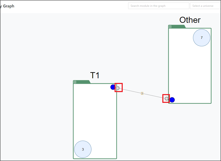
And then selecting all the modules from the window and clicking OK .
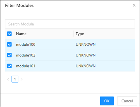
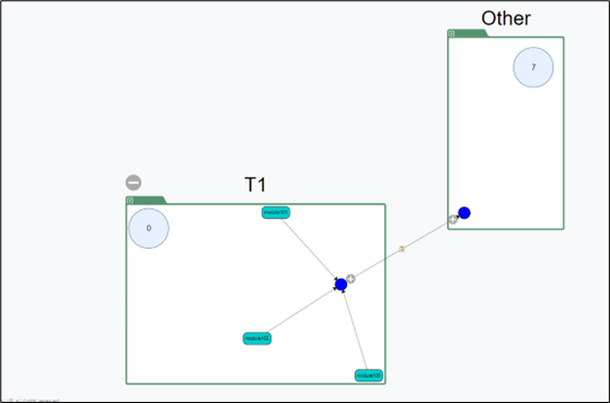
Since all the modules inside the taxonomy are expanded the module count in the circle becomes 0
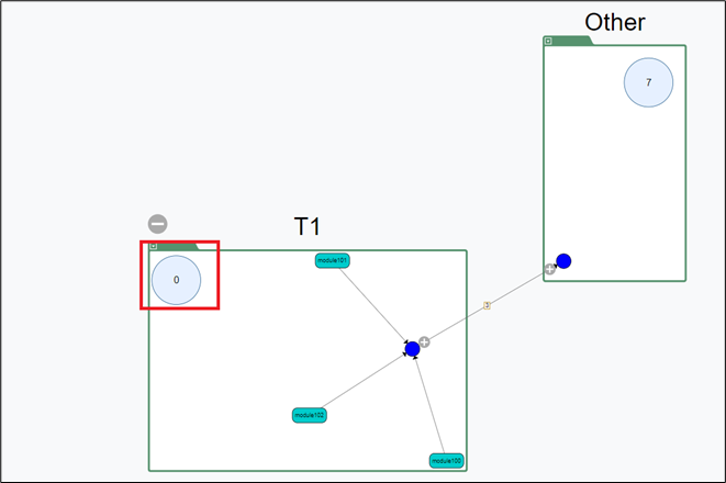
The above graph shows that there is no internal relation between module100, module101 and module102 but they have external connections to the other modules in the remaining taxonomies in the project. This is indicated by the connecting lines to the blue circle.
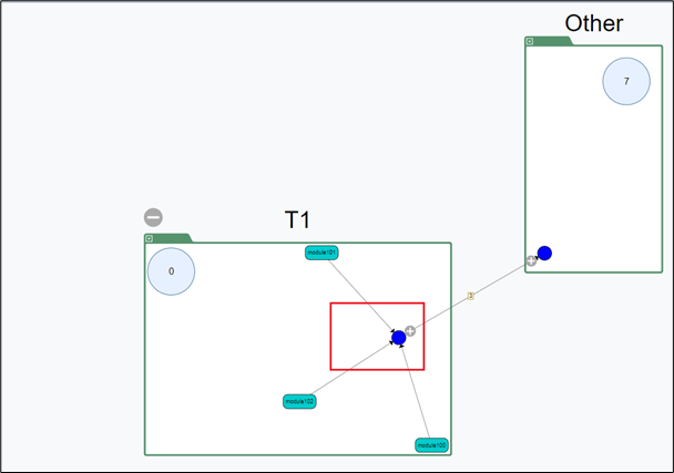
Instead of expanding all internal and external connections at once, you can expand either the incoming or outgoing connection by right-clicking the blue button on the edge of the taxonomy.
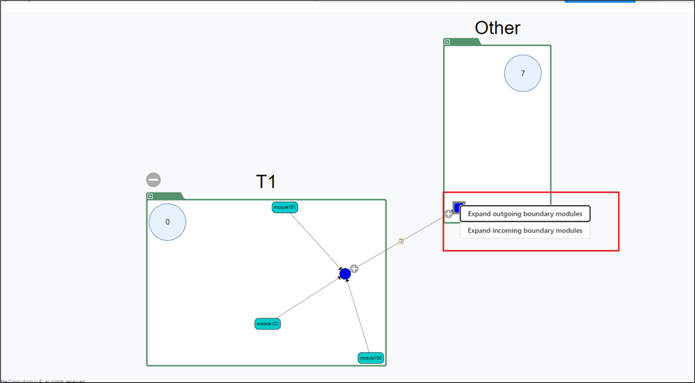
This will selectively expand either the outgoing modules or the incoming modules.
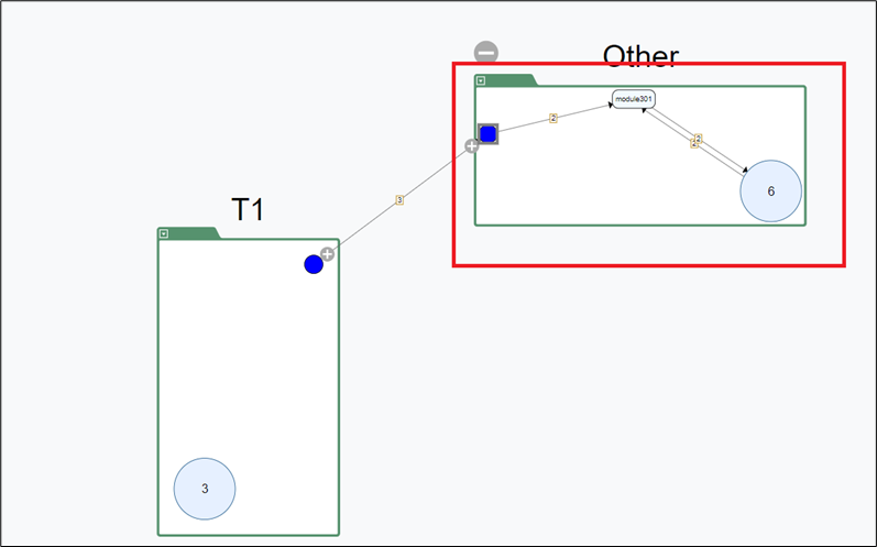
Right-clicking on the expanded module displays some features, for example:
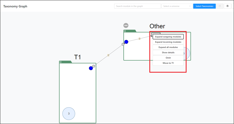
-
Expand outgoing modules: Expands all outgoing modules from the expanded module.
-
Expand incoming modules: Expands all incoming modules into the expanded module.
-
Expand all modules: Expands all modules (incoming + outgoing)
-
Show Details: Shows the details of the modules with the link to the Mining UI and the outgoing and incoming dependencies.
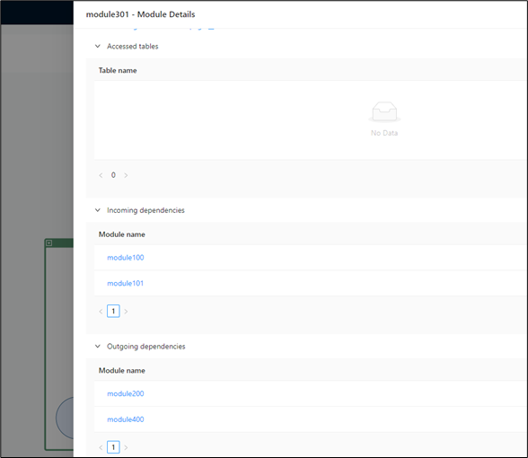
-
Omit: Temporarily removes the module from the graph along with its module relation to other modules.
-
Move: Moves the module to other taxonomies.
Expand connections
You can also expand taxonomies from the unexpanded module count circles by right-clicking them.
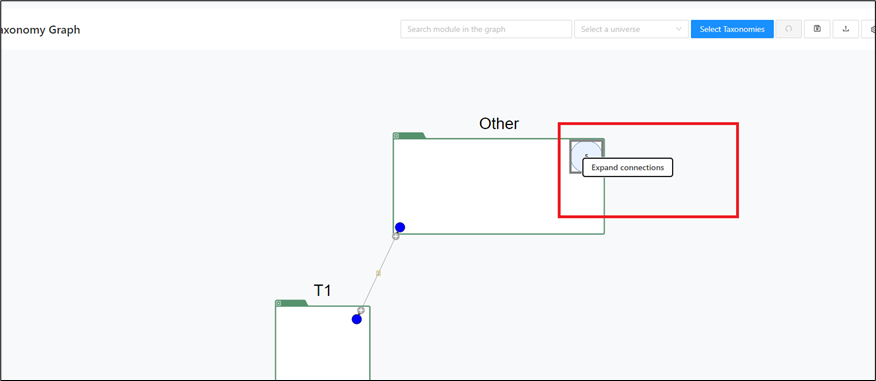
Collapse taxonomies
Taxonomies can be collapsed by clicking on the collapse icon of an already expanded taxonomy.
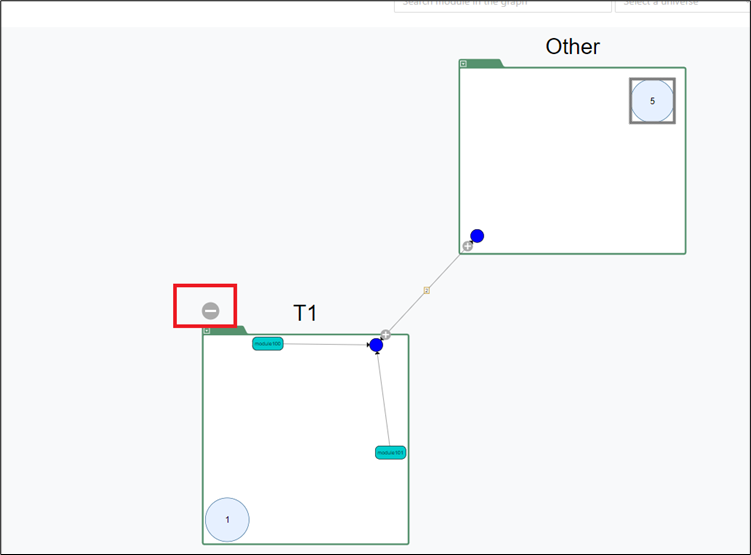
Right-click on taxonomies
Right-clicking on taxonomies opens the options to rearrange the expanded modules or render the taxonomies not displayed currently on the page.
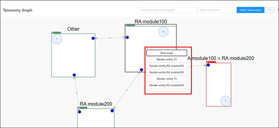
Right-click on empty space
These options help you adjust the graph display.
Right-clicking on an empty space displays the following options:
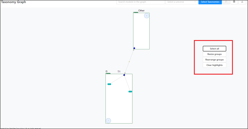
-
Select all: Selects all taxonomies.
-
Resize groups: Is used for resizing.
-
Rearrange groups: Is used for rearranging the taxonomies if the connecting lines/edges overlap.
-
Clear highlights: Clears all existing highlights, for example, after searching for a module in the search bar.
Highlight call chain
To analyze the dependencies between modules and display the call chain of modules in a taxonomy, right-click on any extended module in the taxonomy and select Highlight Call Chain.
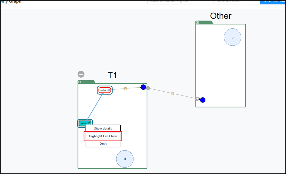
The connection between the selected module and the parent/child module(s) is highlighted.
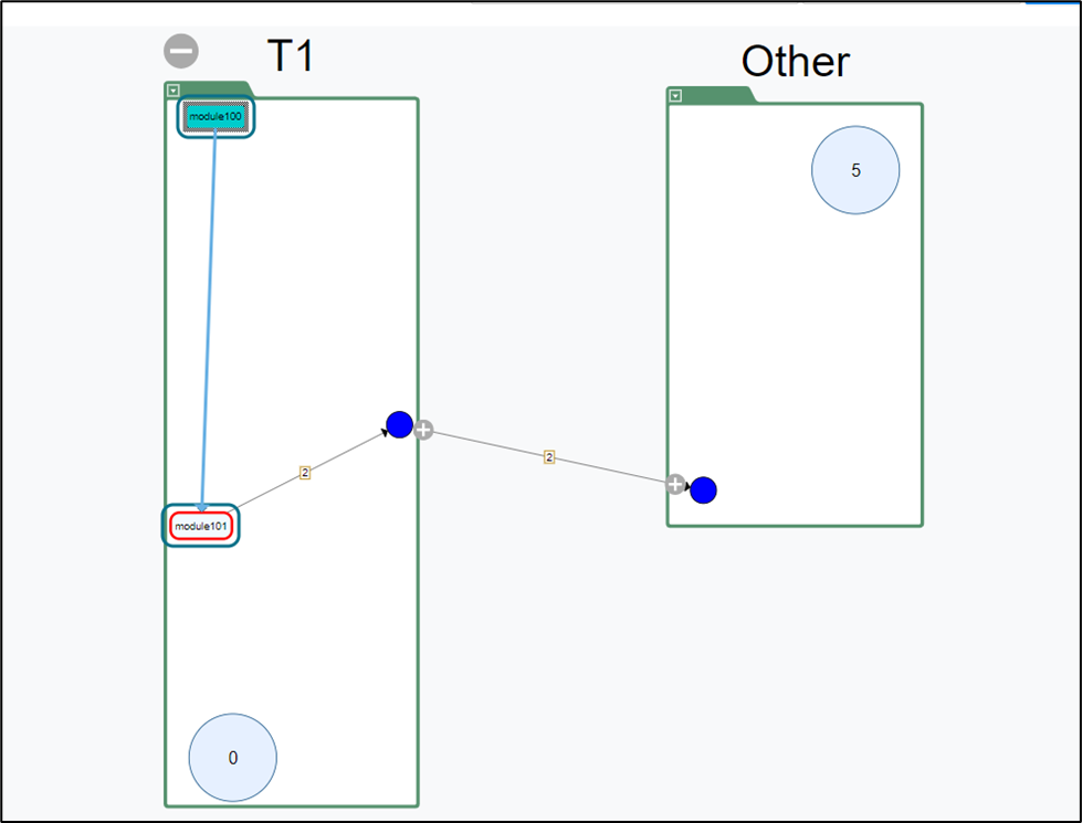
Set future state
To support taxonomy planning, use Set future state to mark a taxonomy with a specific state so you can return later and continue editing.
To do this, proceed as follows:
Step 1:
Right-click anywhere in the taxonomy and select Set future state from the context menu.
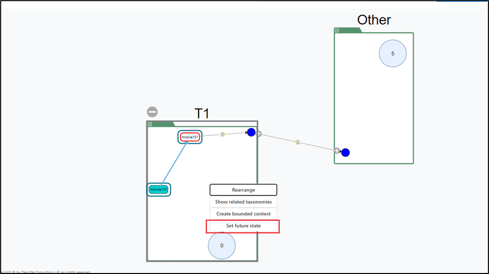
Step 2:
A pop-up window will appear. Select an appropriate option from the drop-down menu.
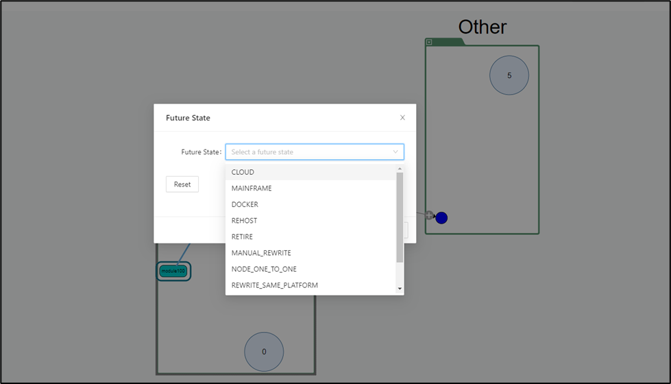
Step 3:
Click OK to confirm your changes.
After a few seconds, the future state is updated and the color of the taxonomy changes from the default green to the color for the option you selected.
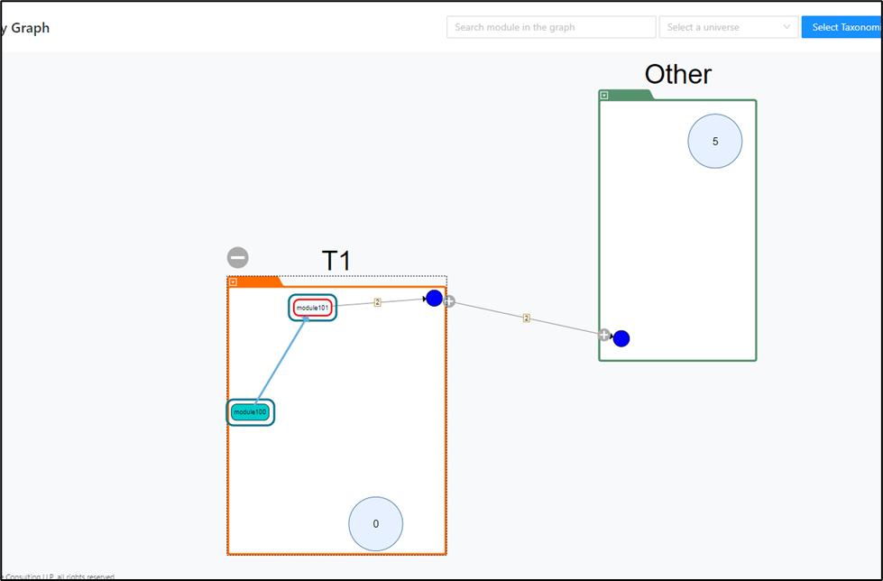
This indicates that the future state has been set. You can change it again whenever needed.
To reset the state to the previous default state, proceed as follows:
Step 1:
Right-click anywhere in the taxonomy and select the Set future state option from the context menu.
Step 2:
A pop-up window will appear. Click Reset and then OK to confirm the changes.
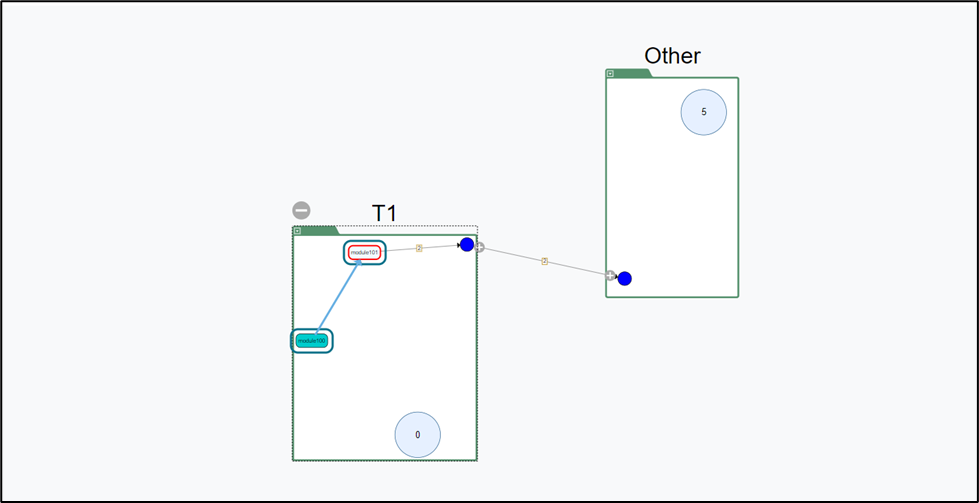
The future state is now updated to the default state.
Decomposition Wizard
Use the Decomposition Wizard to generate decomposition candidates by using the directed Louvain algorithm. This workflow helps you identify candidate clusters based on the imported module landscape before you manually refine bounded contexts. Use it when you want an algorithmic starting point for decomposition rather than building every context by hand.
For this guide, work in Project > Test 3 and open Decomposition > Decomposition Wizard.
The initial wizard view shows the Louvain tab with two accordion steps.
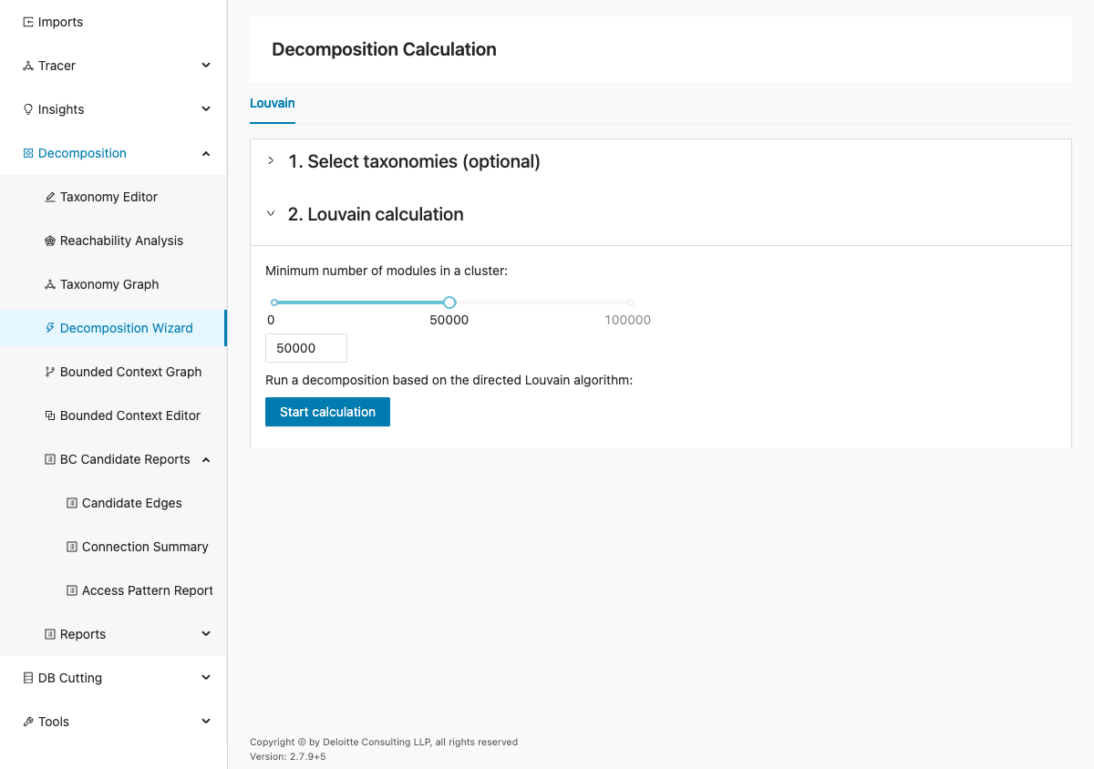
The page contains a single Louvain tab with two steps:
- Select taxonomies (optional)
- Louvain calculation
In Project > Test 3, the taxonomy list may be empty depending on your imported data. Continue with the Louvain calculation even if no taxonomy is selected.
Info
Before you run this workflow, ensure project data was imported successfully (schema, modules, module relations, and queries).
Run the Louvain calculation
This step starts the actual clustering run and applies the Louvain settings to the current project data. The selected parameters affect how many modules are grouped together and whether small clusters are retained. Review the inputs before running the calculation so the resulting candidates are easier to interpret.
To run the calculation in Project > Test 3:
- Open Decomposition > Decomposition Wizard.
- Expand Select taxonomies (optional). If taxonomies are listed, select the relevant entries and click Next. If none are listed, continue to the next step.
- Expand Louvain calculation and set Minimum number of modules in a cluster by using the slider or numeric input.
- Keep the default value unless you have a specific clustering target. In this scenario, use
50000. - Click Start calculation.
Expected output:
- A Decomposition calculation output panel appears below the wizard controls.
- The panel shows the generated result state for Project > Test 3.
Verify the result and continue
After the calculation finishes, review the output carefully before moving on to later decomposition steps. The result tells you whether the current settings produced usable candidates or whether you need to adjust the thresholds and rerun the workflow. Treat this verification step as the handoff from algorithmic grouping to manual context refinement.
After clicking Start calculation, review the output panel before moving to the next feature.
In the previously inspected state, the panel showed:
No taxonomy found as result of decomposition calculation !
The screenshot below shows that output layout.
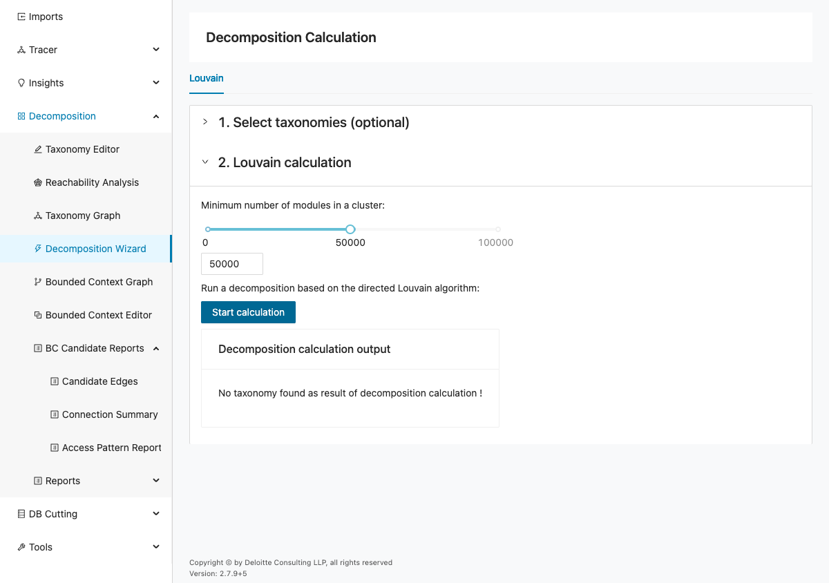
If your Test 3 run generates candidates, continue with Bounded Context Editor to convert selected taxonomies into bounded contexts.
If your run does not generate candidates, reduce Minimum number of modules in a cluster, rerun the calculation, and recheck the output panel.
Bounded Context Graph
The Bounded Context Graph visualizes bounded contexts and module relationships. Bounded contexts can be exported from Mining or generated in Decompose.
For this workflow, use Project > Test 3 and open Decomposition > Bounded Context Graph.
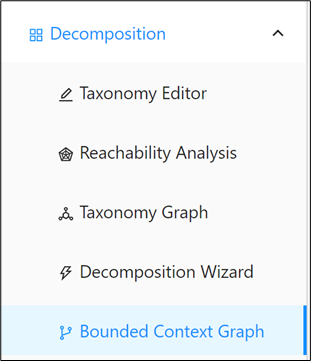
Use this page to inspect cross-context dependencies and refine context boundaries before reviewing BC candidate reports.
Quick start: search and filter contexts
The quickest way to work in the graph is to narrow the visible context set before making any changes. Searching and filtering reduce visual noise and make it easier to focus on the modules or contexts relevant to the current review. Start here whenever the graph is too dense to inspect comfortably.
Step 1: Search for a module in the search field.
Expected output: matching bounded contexts are highlighted with a dark border.
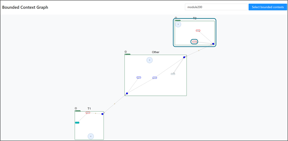
Step 2: In the context list, select only the bounded contexts you want to display.
Expected output: selected contexts remain visible and unselected contexts are hidden.

Step 3: Select contexts one-by-one or use the checkbox beside Name to select all.
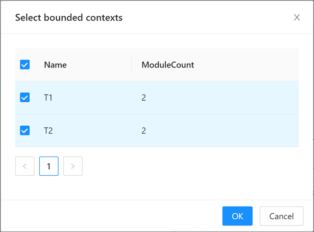
Understand graph elements
Before you move modules or interpret edges, make sure you understand what the graph is showing. The labels, boundaries, and edge patterns all carry meaning that affects decomposition decisions. This section summarizes the visual elements you will use throughout the graph workflow.
The graph shows bounded context names and the boundary modules shared across contexts.
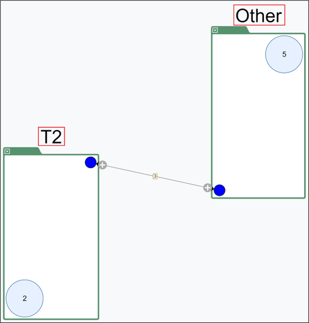
Boundary module relationships are represented by edges between contexts.
Inspect connections in the drawer
The drawer is the detailed inspection area for a specific relationship between two contexts. It lets you review the modules involved, assess the impact of moving them, and preview how boundary changes affect connectivity. Use it when the high-level graph indicates a relationship that needs a closer look.
Step 1: Click an edge between two contexts.
Expected output: a drawer opens showing boundary modules and connection details.
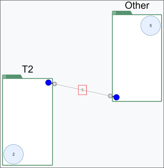
Step 2: Review module names, internal/external connections, and preview impact if modules are moved.
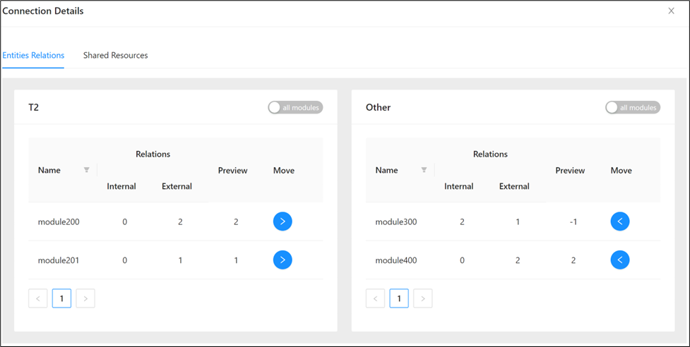
Step 3: Use the drawer filter to narrow the module list.
Expected output: only matching modules remain visible in the drawer list.
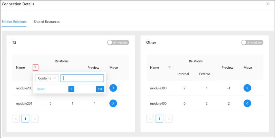
Step 4: Use and to move modules between contexts.
Expected output: module ownership updates and connection previews reflect the new assignment.
Step 5: Toggle all modules when you need to inspect more than boundary modules.
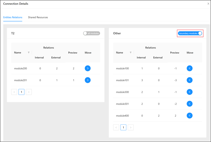
If all modules is disabled, boundary modules and all modules are currently the same set.
Expand contexts and module-level relations
Expanding contexts exposes the individual modules and connections hidden behind the summary circles. This deeper view helps you distinguish between broad context-level coupling and a small number of specific module dependencies. Use it when you need to understand why two contexts appear connected.
Unexpanded modules are shown as module-count circles.
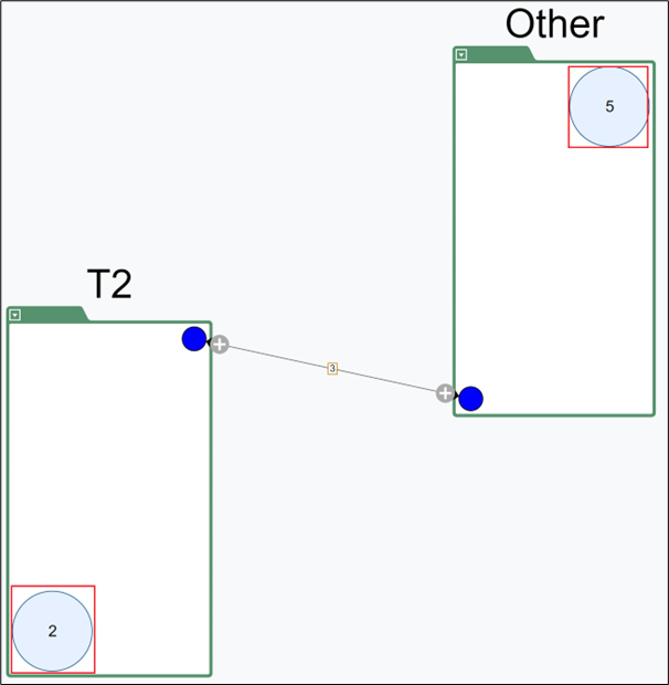
Step 1: Click the icon on an edge to expand contexts.
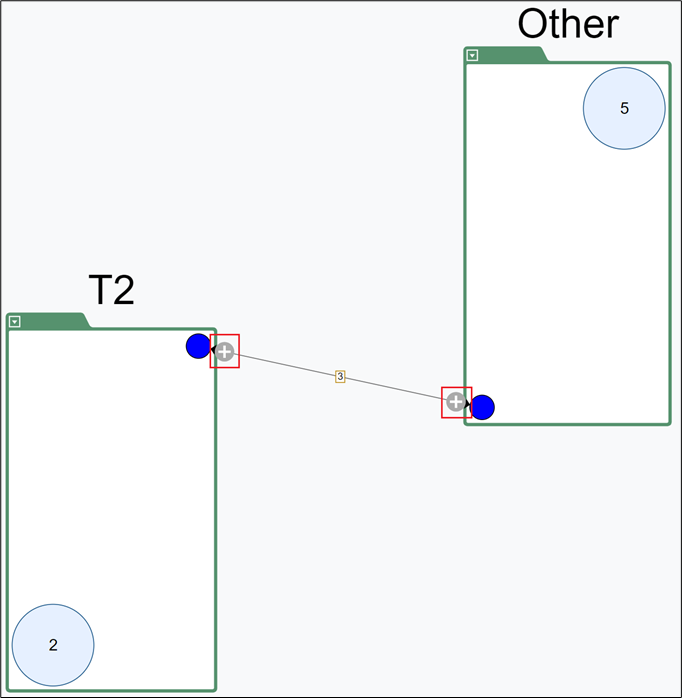
Step 2: In the selection dialog, choose modules and click OK.
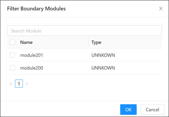
Step 3: Review the expanded result.
Expected output: expanded modules are shown, and fully expanded context circles can show a module count of 0.
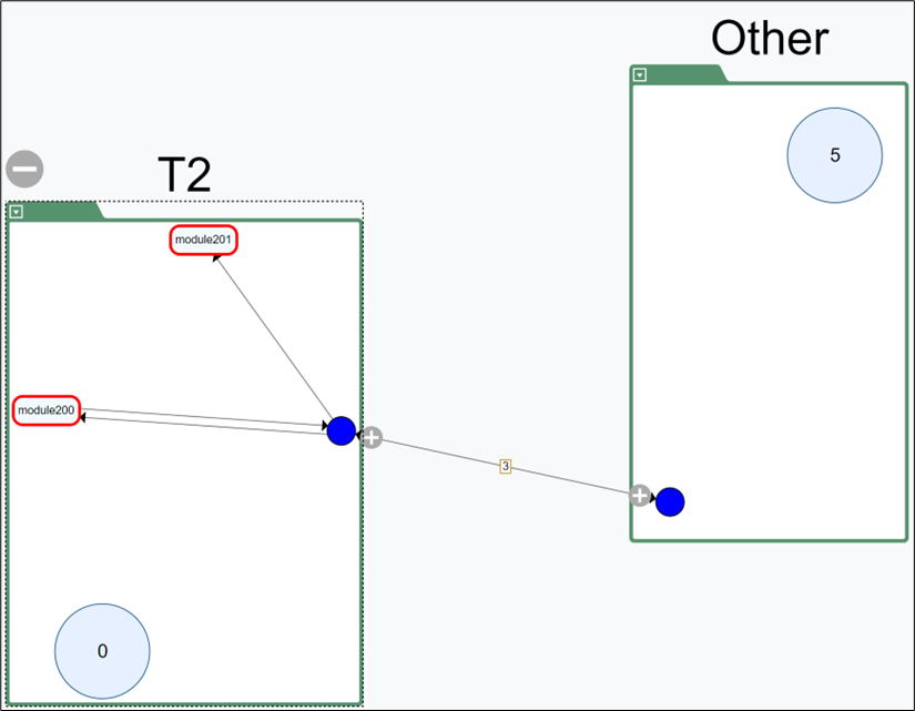
The graph can show modules with no internal links but external connections to other contexts.
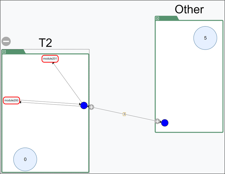
Step 4: To expand selectively, right-click the blue edge control and choose incoming or outgoing expansion.
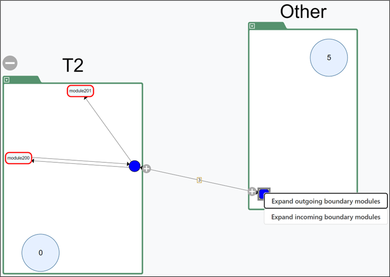
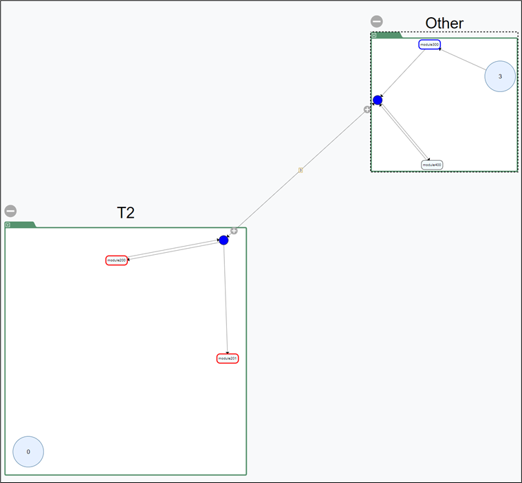
Step 5: Right-click an expanded module to use advanced options.
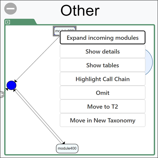
- Expand outgoing modules: expands outgoing dependencies.
- Expand incoming modules: expands incoming dependencies.
- Expand all modules: expands incoming and outgoing dependencies.
- Show Details: opens detailed module metadata and dependency information.
- Omit: temporarily removes the module and related lines.
- Move: moves the module to another context.
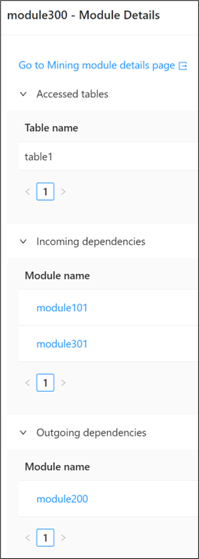
Step 6: You can also expand from unexpanded module-count circles by right-clicking a circle.
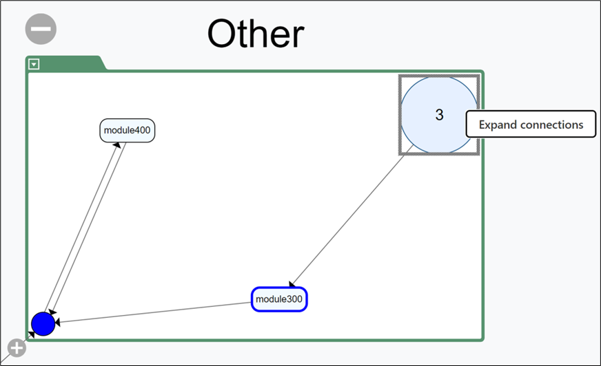
Step 7: Collapse an expanded context by clicking .
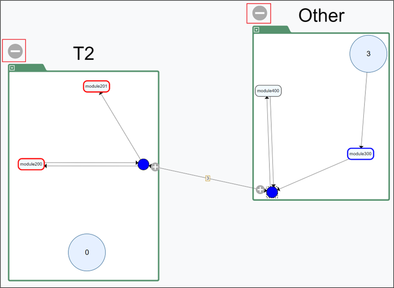
Adjust layout and clear highlights
Layout controls help you keep the graph readable as you refine context boundaries and run repeated searches. They are useful after expanding modules, moving ownership, or filtering the view several times in one session. Use these actions to reset the visual state before continuing your review.
Right-click empty graph space to open layout controls.
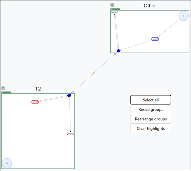
- Select all: selects all visible contexts.
- Resize groups: resizes displayed groups.
- Rearrange groups: rearranges contexts when edges overlap.
- Clear highlights: clears current search highlights.
After refining contexts in the graph, continue with BC Candidate Reports to review Candidate Edges, Connection Summary, and Access Pattern output.
Bounded Context Editor
The Bounded Context Editor is where you turn taxonomy work into explicit bounded contexts that can be reviewed in later graph and report pages. It provides a controlled step between exploratory taxonomy analysis and more formal decomposition outputs. Use this page when you are ready to promote selected taxonomies into context candidates.
Info
Before you use this page, create a client and project, then upload schema, modules, queries, taxonomy, and module-relations CSV files.
For this workflow, use Project > Test 3. Open Decomposition > Bounded Context Editor and switch to the Taxonomy To Context tab.
Convert taxonomies to bounded contexts
This workflow copies selected taxonomies into bounded contexts so they can be analyzed independently of the original taxonomy set. It is the main transition point from taxonomy-based grouping to context-based decomposition. Complete these steps after you are satisfied with the taxonomies you want to promote.
Step 1: Scroll to the taxonomy list and identify the taxonomies you want to convert. You can move taxonomies one-by-one or as a batch.
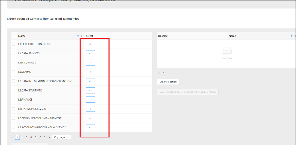
Step 2: To move one taxonomy, click -> on its row.
Expected output: the selected item appears in the right-side selection pane.
The selected bounded context appears in the pane on the right.
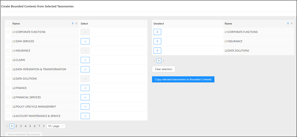
Step 3: (Optional) Use list controls to narrow the selection set before conversion.
Use filters, sorting, and pagination in the taxonomy list.
Expected output: the list updates immediately so you can target the correct taxonomy set for Test 3.
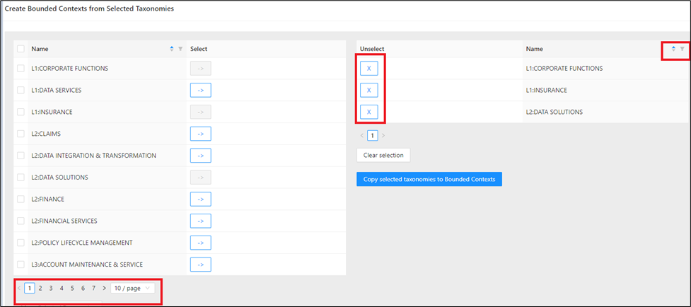
Step 4: To move all visible taxonomies, select the master checkbox and click Move Selected Taxonomies.
Expected output: all checked taxonomies move into the right-side pane.
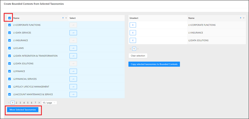
Step 5: If you need to adjust the selection:
- Click next to an item in the right pane to remove one taxonomy.
- Click Clear Selection to remove all selected taxonomies.
Expected output: removed entries return to the left list.
Step 6: When the right pane contains your final Test 3 selection, click Copy selected taxonomies to Bounded Contexts.
Expected output: selected taxonomies are copied and become available under Select Context.
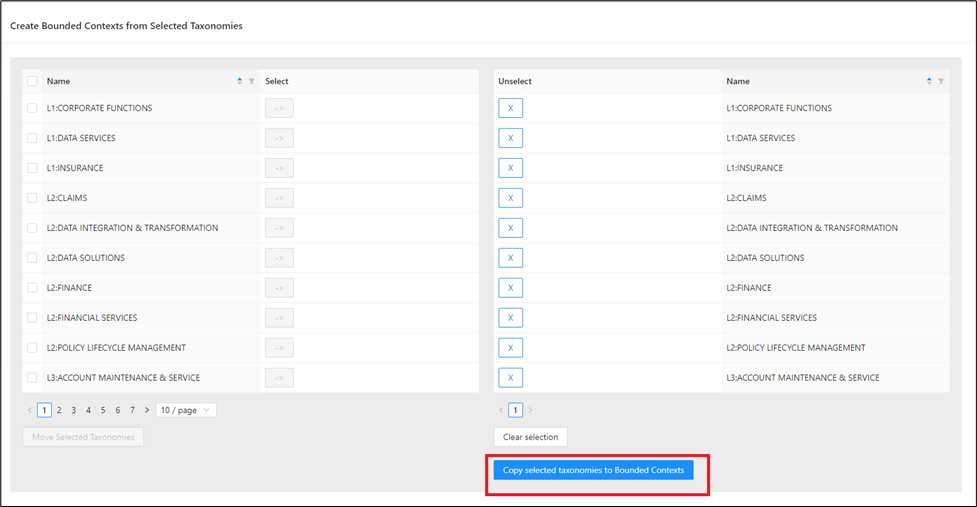
Step 7: Open the Select Context tab and confirm the copied contexts are listed.
Expected output: new bounded contexts are available for graph analysis.
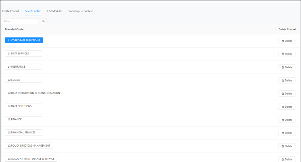
Continue with Bounded Context Graph to inspect and refine context boundaries.
BC Candidate Reports
Use BC Candidate Reports to validate bounded context candidates generated and refined in earlier steps. These reports turn the current decomposition state into tables that are easier to review, compare, and export. Use them when you need evidence for boundary decisions before finalizing bounded contexts.
Before running these reports, complete:
Open the report area from Decomposition > BC Candidate Reports. Each report includes download actions, sortable table columns, and pagination controls.
Candidate Edges
The Candidate Edges report highlights cross-context relationships that may indicate coupling between proposed bounded contexts. It is useful for spotting boundaries that still need refinement after graph-based editing. Review this report when you want to understand where modules still connect across candidate contexts.
Open the Candidate Edges page from Decomposition > BC Candidate Reports > Candidate Edges.
The screenshot below shows the Candidate Edges report layout.
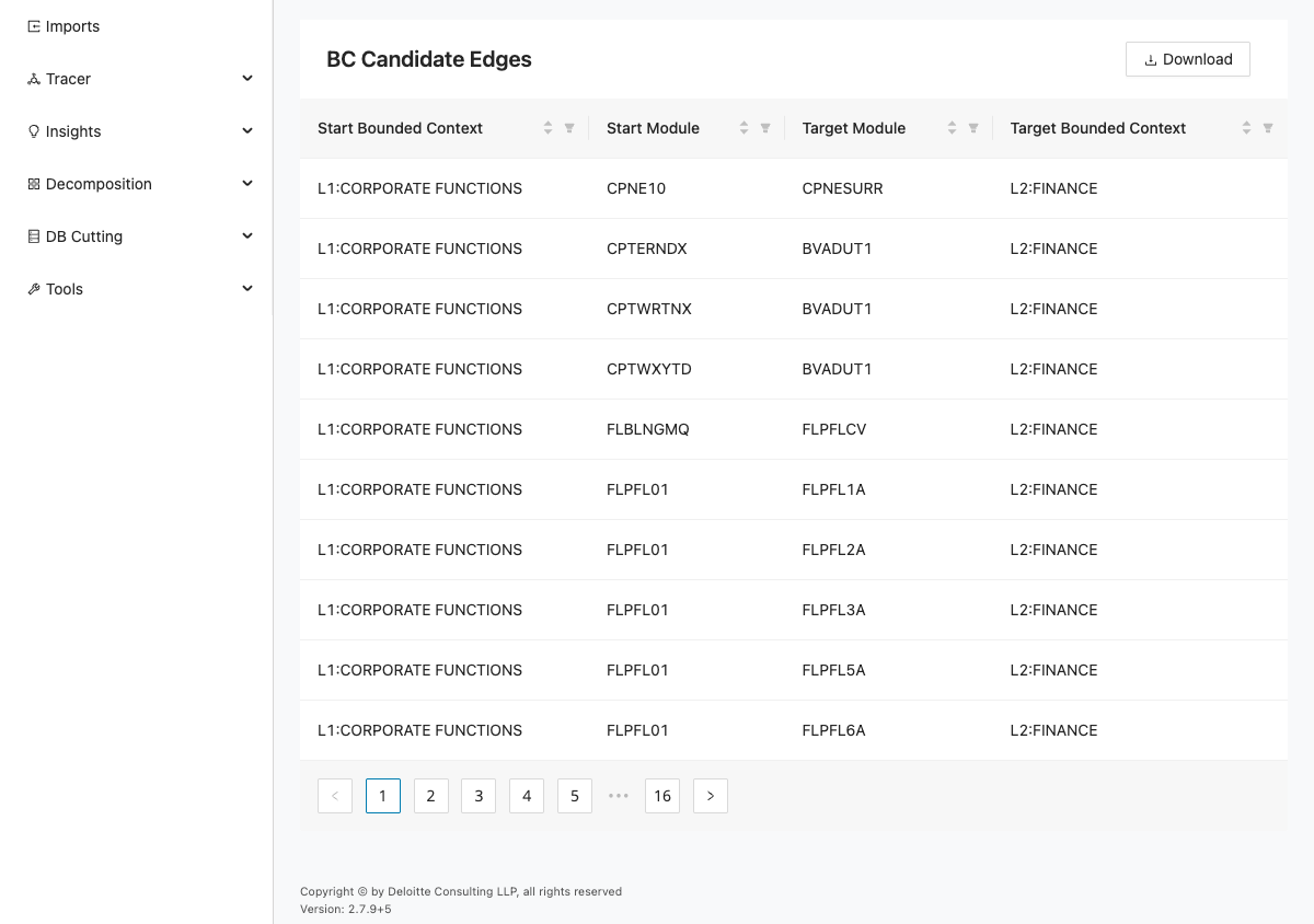
This report shows candidate relationships between modules and bounded contexts. The page contains Download and a table with the following columns:
| Column | Description |
|---|---|
| Start Bounded Context | Source bounded context for the candidate relationship. |
| Start Module | Source module for the candidate relationship. |
| Target Module | Target module for the candidate relationship. |
| Target Bounded Context | Target bounded context for the candidate relationship. |
The table headers are sortable and the standard pagination controls are shown below the table.
- The table is populated with candidate edges after decomposition and bounded context conversion.
- Each row identifies a source context/module and target context/module pair.
- Live validation captured 10 table rows.
Use this report to identify unexpected cross-context edges. If you see misclassified relationships, return to Bounded Context Graph and move modules to reduce unnecessary cross-context dependencies.
Connection Summary
The Connection Summary report aggregates context-to-context traffic so you can identify heavily connected pairs at a glance. It helps you prioritize which boundaries deserve a closer architectural review. Use it when the detailed edge list is too granular and you need a higher-level picture of coupling.
Open the Connection Summary page from Decomposition > BC Candidate Reports > Connection Summary.
The screenshot below shows the Connection Summary report layout.
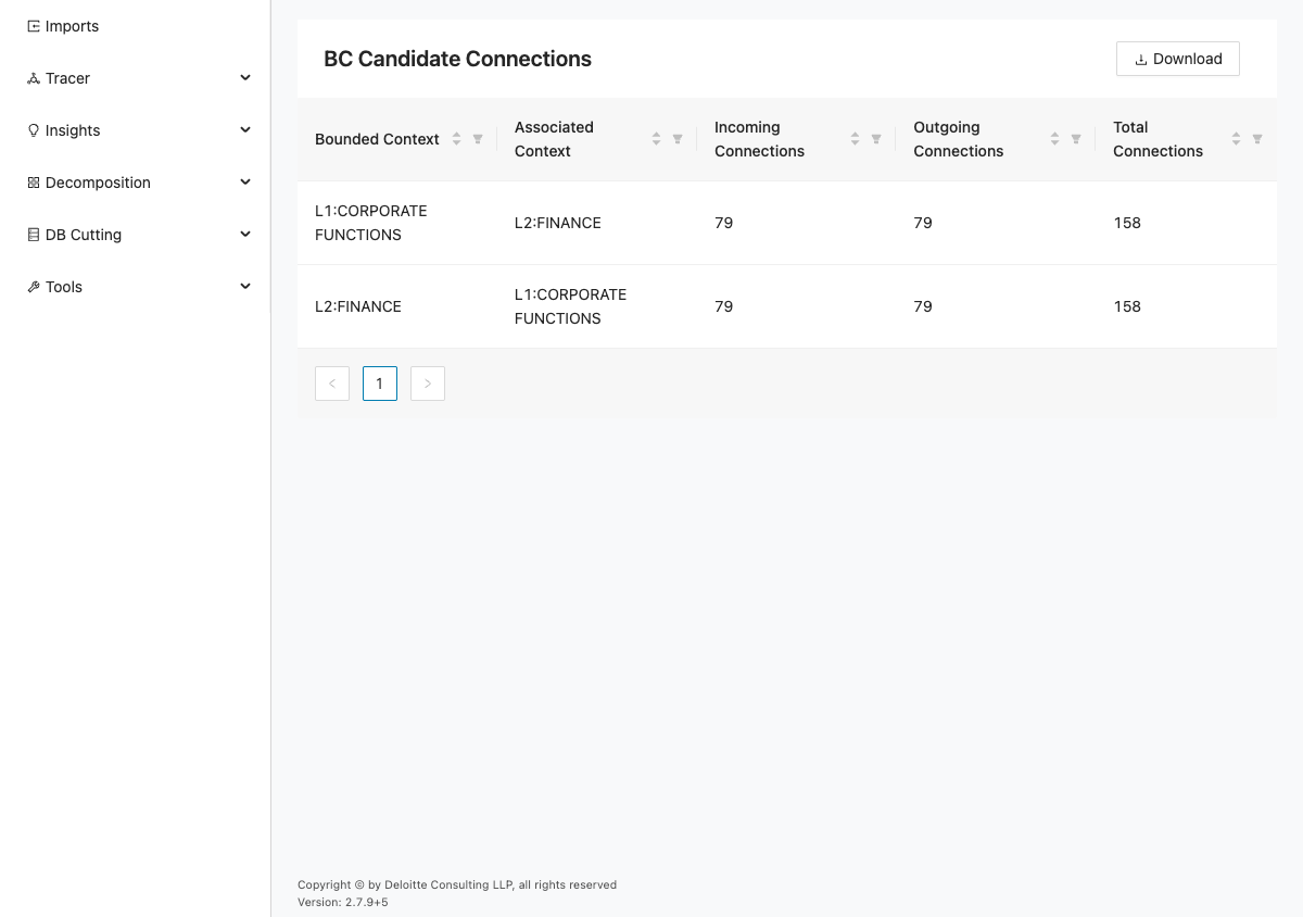
This report provides a bounded-context summary of incoming and outgoing connections. The page contains Download and a table with the following columns:
| Column | Description |
|---|---|
| Bounded Context | Bounded context shown in the summary. |
| Associated Context | Related context paired with the bounded context. |
| Incoming Connections | Number of incoming connections for the context pair. |
| Outgoing Connections | Number of outgoing connections for the context pair. |
| Total Connections | Total number of connections for the context pair. |
The table headers are sortable and standard pagination controls are shown below the table.
- The table is populated with bounded context pairs and connection counts.
- Total Connections helps prioritize contexts that need boundary refinement.
- Live validation captured 2 table rows.
Use this report to find heavily coupled context pairs. Then revisit Bounded Context Graph to inspect and adjust module placement on the related edges.
Access Pattern Report
The Access Pattern Report brings database access behavior into the bounded context candidate review. It shows where modules within a candidate context read from or write to shared tables and columns. Use it to confirm ownership assumptions and to find data hotspots that may require additional design work.
Open the Access Pattern Report page from Decomposition > BC Candidate Reports > Access Pattern Report.
The screenshot below shows the Access Pattern Report layout.
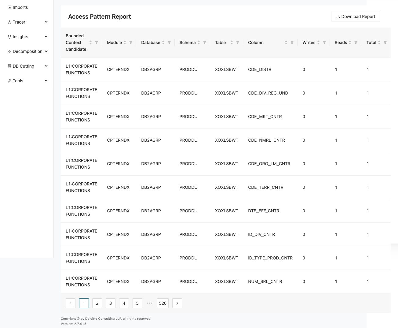
This report shows data-access activity associated with bounded context candidates and modules. The page contains Download Report and a table with the following columns:
| Column | Description |
|---|---|
| Bounded Context Candidate | Bounded context candidate tied to the access record. |
| Module | Module tied to the access record. |
| Database | Database for the access record. |
| Schema | Schema for the access record. |
| Table | Table for the access record. |
| Column | Column for the access record. |
| Writes | Number of writes recorded. |
| Reads | Number of reads recorded. |
| Total | Total reads and writes recorded. |
The table headers are sortable and standard pagination controls are shown below the table.
- The table is populated with data access records (reads/writes/total) by candidate context and module.
- Shared table access across multiple contexts is visible in the Database, Schema, and Table columns.
- Live validation captured 10 table rows.
Use this report to find data ownership conflicts and shared-table hot spots. If a context boundary looks incorrect, go back to Bounded Context Editor or Bounded Context Graph, adjust contexts, and rerun the reports.
Reports
Use Reports to review bounded-context interconnections, modules that are not part of a bounded context, and the visual context graph. These pages provide exportable views of the current decomposition state so you can validate decisions outside the graph editors. Use them when you need a report-oriented summary of context structure and gaps.
Connected Context
The Connected Context report focuses on the relationships between bounded contexts and the modules that create those links. It is useful for understanding where context boundaries still depend on each other and for reviewing those interconnections in a table-based format. To use it, export the Bounded Contexts and modules file from Mining and import it into Unified Cutter, or move taxonomies to contexts from Taxonomy Editor.
In the left navigation panel, navigate to Decomposition > Reports > Connected Context.
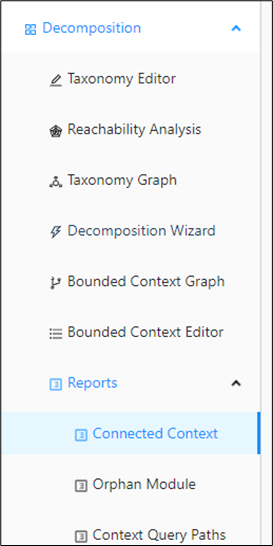
The connected context report is displayed as a table:
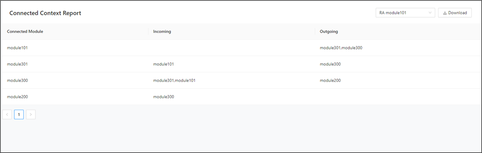
It shows the connected modules in the selected bounded context together with the incoming and outgoing module information.
Use the dropdown to switch between different contexts.
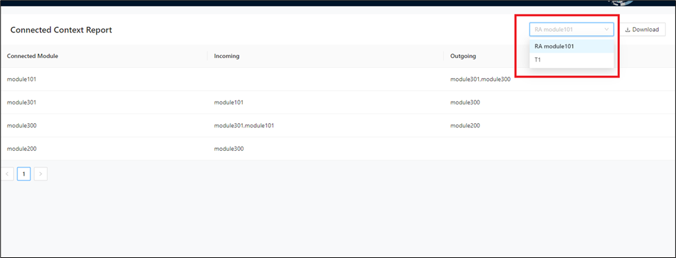
Click Download to download the report in a file.
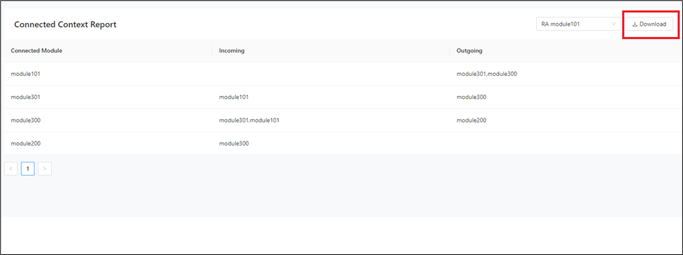
Orphan Module
The Orphan Module report shows modules that are currently outside the selected bounded context and may still need classification. It helps you identify decomposition gaps and leftover modules that are not yet represented in the target structure, making it useful when you want to find work that remains before a context model is complete. To use this report, export the Bounded Contexts and modules file from Mining and import it into Unified Cutter, or move taxonomies to contexts from Taxonomy Editor.
In the left navigation panel, navigate to Decomposition > Reports > Orphan Module.
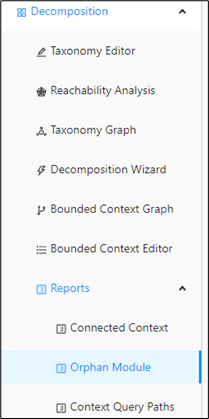
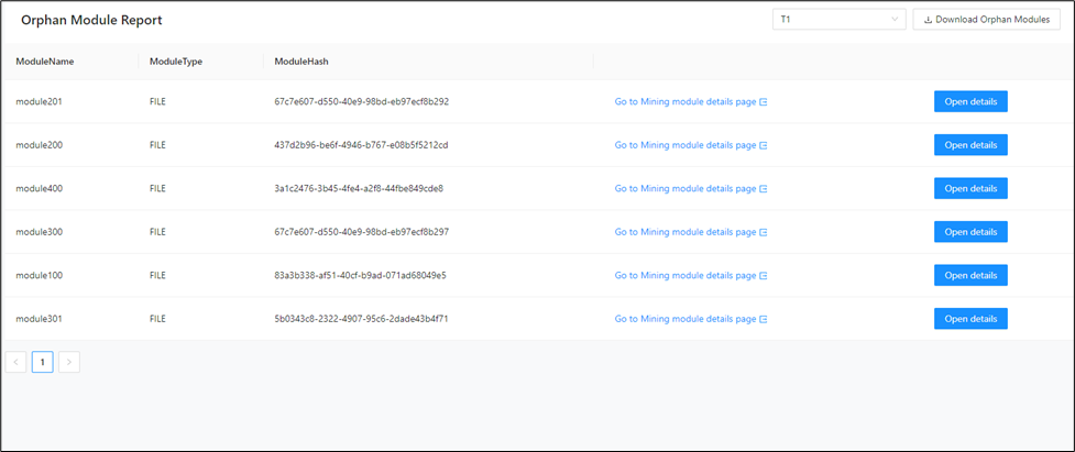
The report is displayed as a table with the module name, type, module hash, link to the Mining UI, and details of the incoming and outgoing dependencies.
Use the dropdown to switch between different contexts.
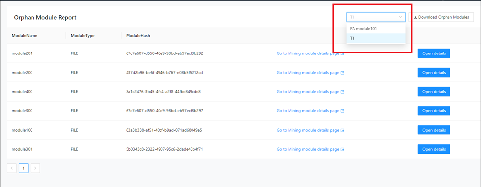
Open Details shows the accessed table, the incoming and outgoing dependencies of the module, and a link to the Mining UI.
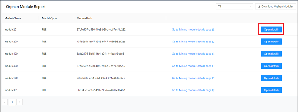
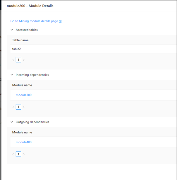
Click Download to download the report in a file.
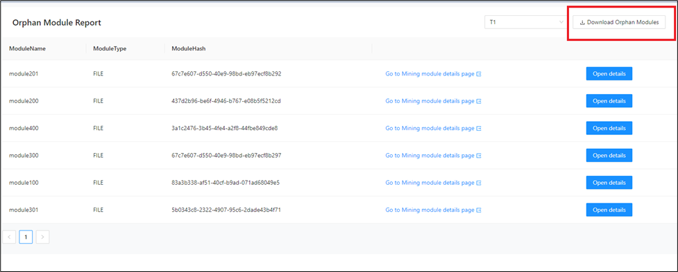
Context Query Paths
The Context Query Paths page combines bounded contexts, modules, and tables into a graph so you can inspect ownership and access behavior together. It is especially helpful when you want to review context structure alongside the database objects each context touches and to make targeted context updates from the graph. To use this page, export the Bounded Contexts and modules file from Mining and import it into Unified Cutter, or move taxonomies to contexts from Taxonomy Editor.
In the left navigation panel, navigate to Decomposition > Reports > Context Query Paths.
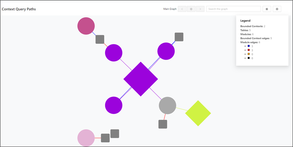
You can zoom in and out of the graph to inspect more bounded-context detail.
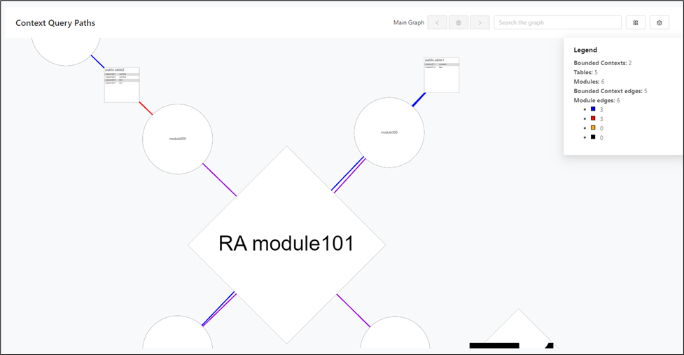
The legend shows the details of the Bounded Contexts along with the number of Read/Write queries, triggers.
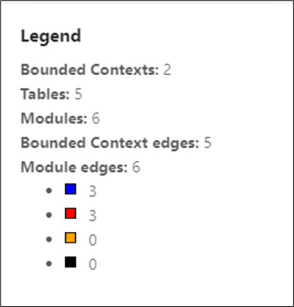
Use the search bar to find a specific module or table.
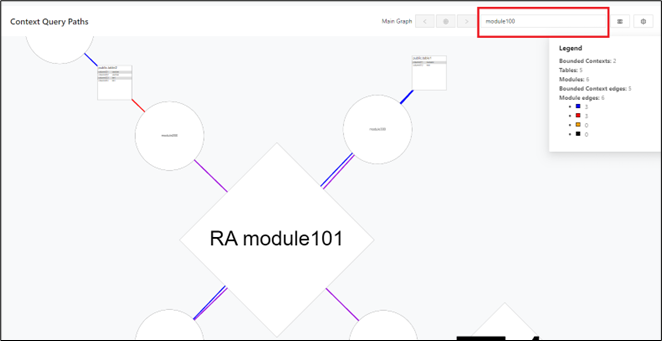
Use the back button or the return-to-main-graph button to navigate back to the main graph.
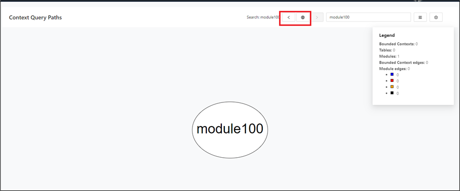
Assign modules to contexts
You can create new contexts and assign modules to the visible contexts from the Context Query Paths graph.
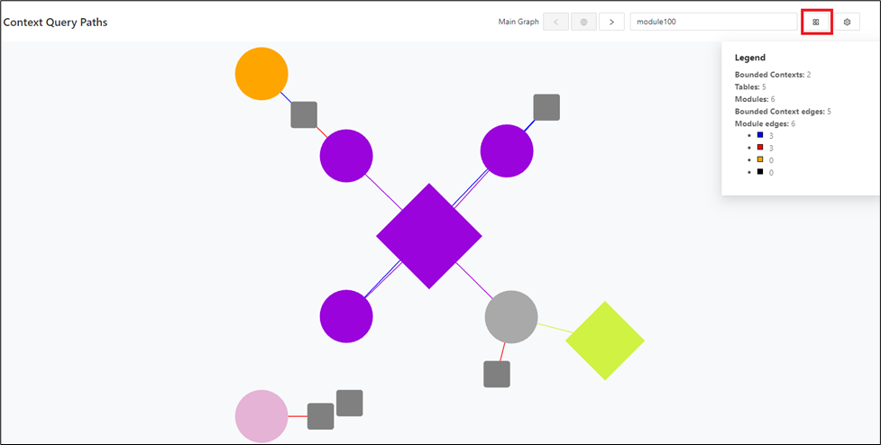
A new context can be created:
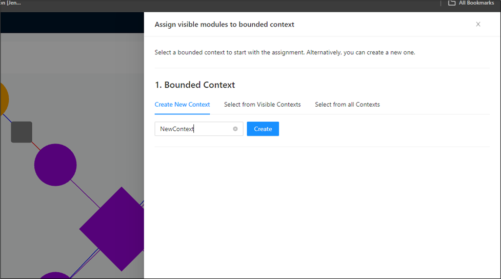
You can select a context from the existing contexts. This list does not include a context created in the previous step:
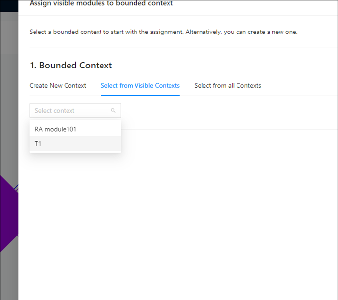
You can select a context from all contexts. This list includes a context created in the previous step:
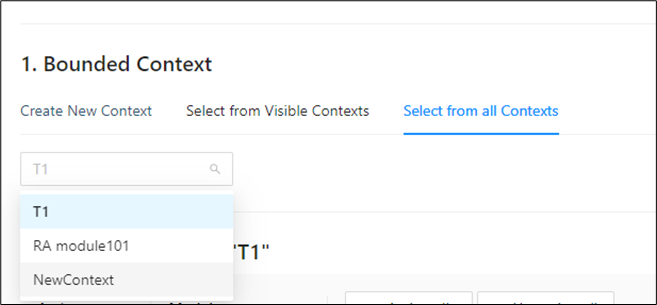
Assign modules to contexts individually by clicking the switches alongside the modules, or assign them all at once by using Assign All.
Unassign modules from contexts individually by clicking the switches alongside the modules, or remove them all at once by using Un-assign All.
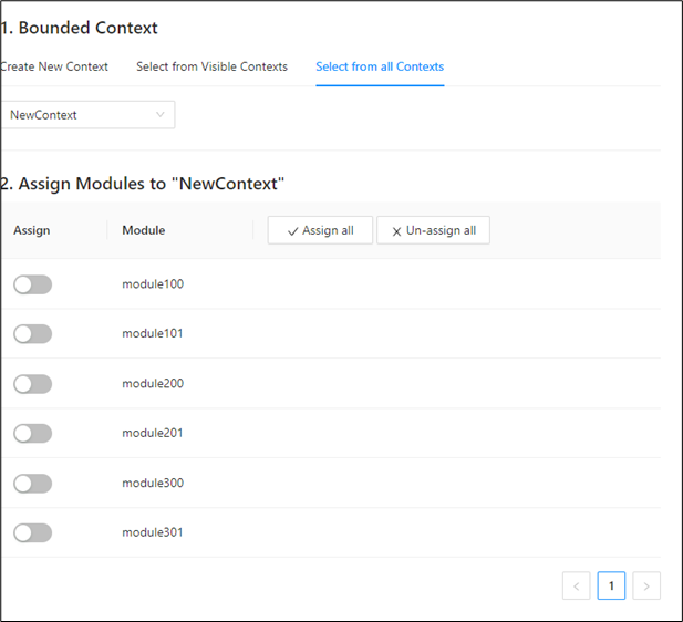
After the assignment, the changes are visible in the graph.
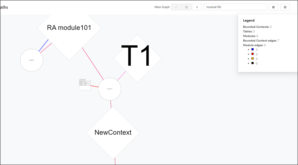
Graph options
Use these options to change how the graph is displayed.
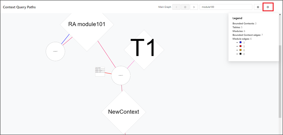
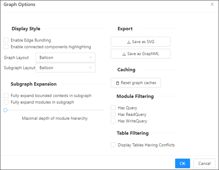
Display style: Highlights the connected edges.
Graph and subgraph layout: Displays the graph and subgraph in four orientations: Balloon, Hierarchical, Organic, and Radial.
Subgraph expansion: Controls how far the subgraph expands. More depth shows more information.
Export: Saves the graph as an SVG or GraphML file.
Caching: Resets caches to prevent incorrect graph display.
Module filtering: Filters the graph by read or write activity, or by query and no-query state.
Graph options for module filtering
-
Has Query
-
Description: Displays modules that have any type of query associated with them.
-
Use Case: Ideal for identifying modules that are actively engaged in querying operations.
-
-
Has ReadQuery
-
Description: Shows modules that specifically have read queries.
-
Use Case: Useful for analyzing modules that are involved in data retrieval operations.
-
-
Has WriteQuery
-
Description: Shows modules that have write queries.
-
Use Case: Best for examining modules that are responsible for data insertion or updates.
-
Table filtering filters tables with conflicts.
Display table options for conflict filtering
-
Display Tables Having Conflicts
-
Description: Visualization of conflicts, including the number of conflicts.
-
Use Case: Useful for identifying the overall conflict landscape.
-
Conclusion
Use the graph and table options to tailor the visualization and conflict analysis to your needs. The object count is displayed for each targeted module.
DB Cutting
The DB Cutting menu provides the functionality at the heart of Decompose. The following section describes the sub-pages that provide the core functionality: Decompose.
Table Decomposer
The Table Decomposer displays the tables that are already connected to the current bounded context. When you start from the legacy graph, the Table Decomposer is already initialized with a set of tables.
Navigate to DB Cutting > Table Decomposer.
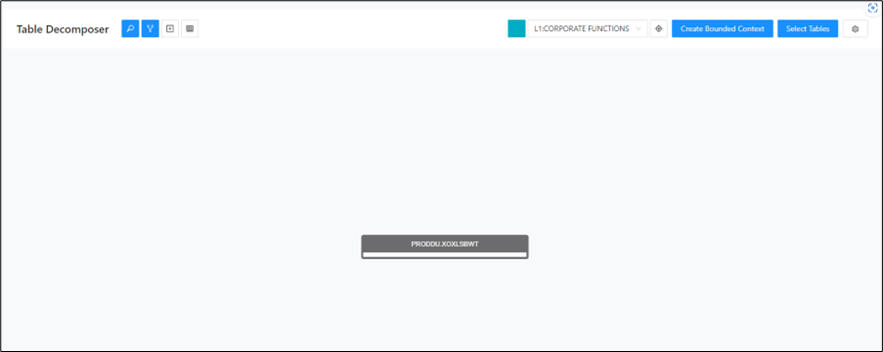
Selecting tables:
Info
The Non-standard Data Access column indicates which tables are in read-only or write-only contexts.
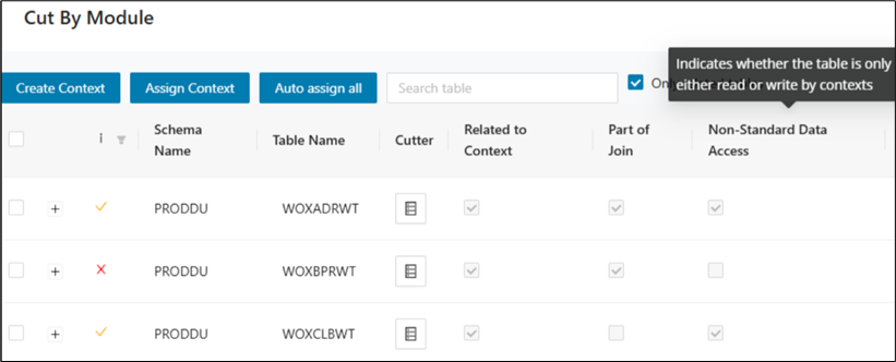
Step 1:
Click Select Tables toward the top right corner of the screen.
Step 2:
Set the filter on Schema Name and the Table Name if required.
Step 3:
Select the required tables and click Show Only Selected .
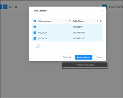
Step 4:
Click Render Graph .
Assign to currently selected Bounded Contexts
Step 1:
Right click on the table and select "Assign to current Bounded Context".
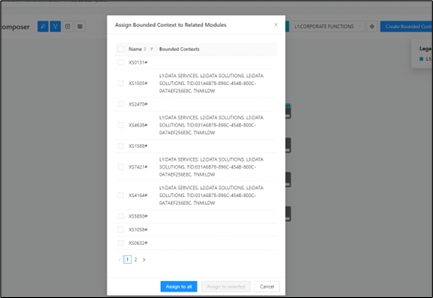
Step 2:
Select the required module that are to be included to the Bounded Context.
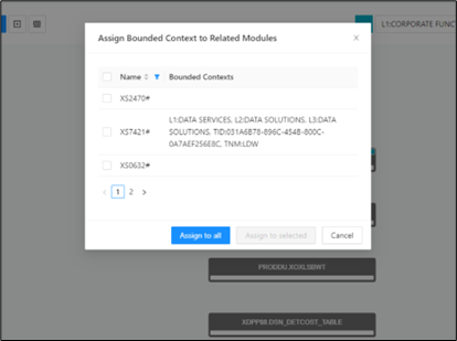
Step 3:
Click Assign to Selected .
Remove Bounded Context:
Step 1:
Right click on the table and select Remove Bounded Context .
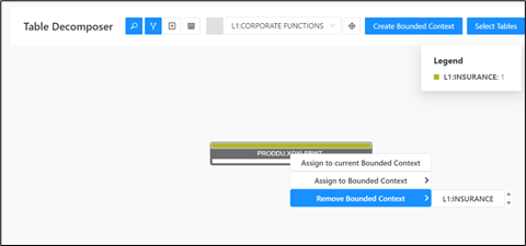
Step 2:
Select the Bounded Context. Bounded Context is successfully removed for the table.
Cut by Module
The Cut by Module view helps you review tables in the context of the modules and bounded contexts that use them. It is designed for conflict resolution and migration-strategy assignment at the column level. Use this page when you want to evaluate ownership decisions table by table while keeping application behavior in view.
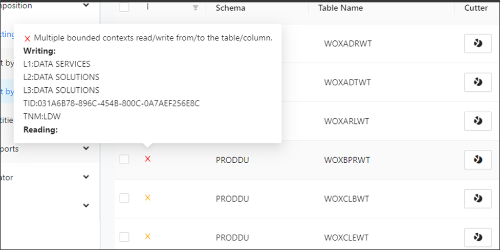
To start cutting by module, import the schema, bounded contexts, modules, and queries, and then resolve conflicts in the Cut by Module view. In that view, review each table and assign the appropriate migration strategy for all columns.
Use Auto Assign All to quickly assign a strategy to the table columns. When you click this button, an appropriate strategy is selected for each column unless the column has conflicts that cannot be resolved automatically. In those cases, you must choose the best strategy.
The general workflow is to first import the schema, then the bounded contexts, modules, and queries, and after that resolve conflicts in the Cut by Module view.
Step 1:
In the left navigation panel, select DB Cutting > Cut by Module.
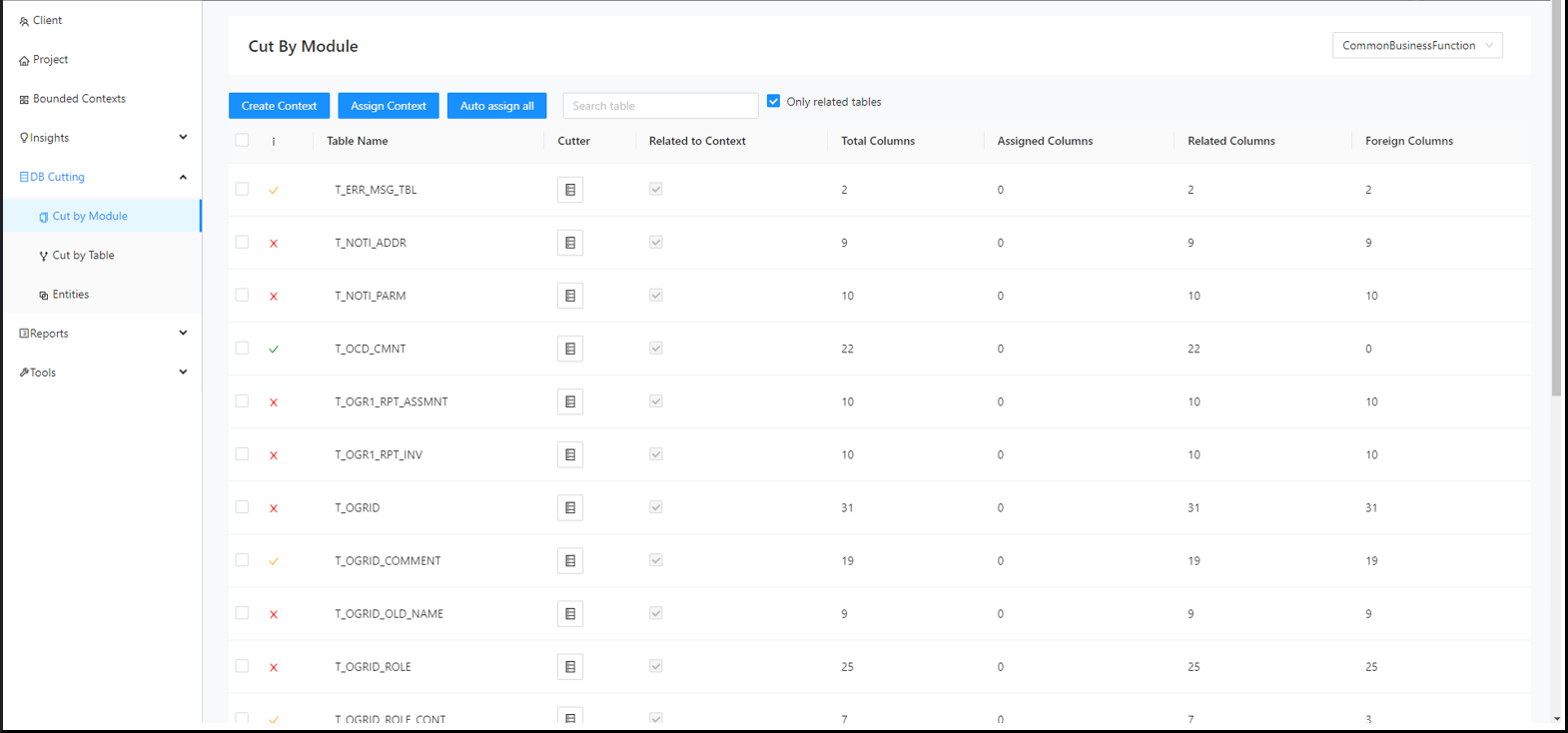
Step 2:
Select a bounded context from the drop-down list in the upper right corner of the page.
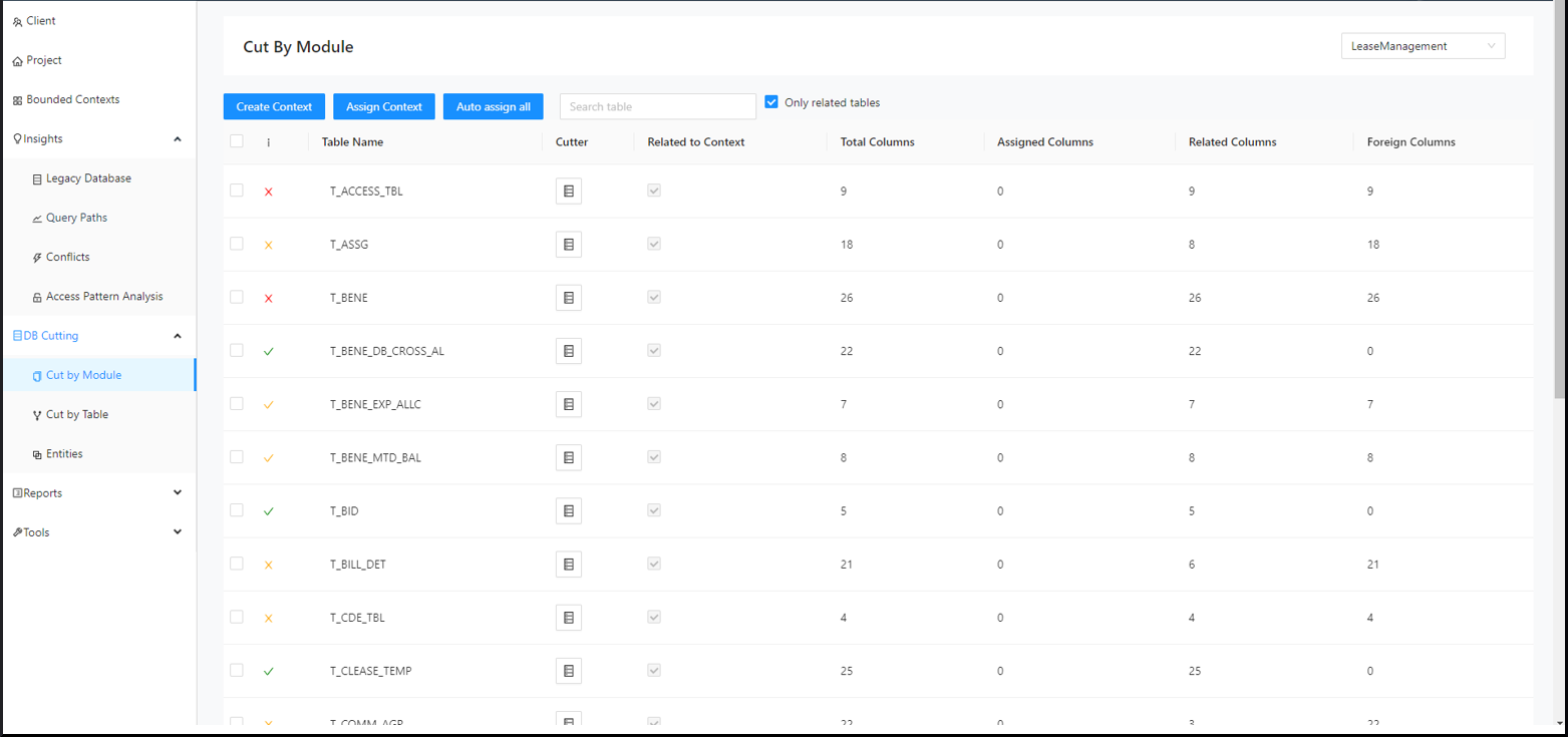
Step 3:
Use the search bar to find the table to cut.
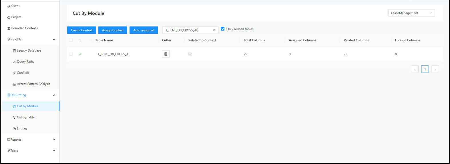
Step 4:
Click on the expand icons beside the tables to display the information about bounded contexts other than the one already selected that are accessing the tables.
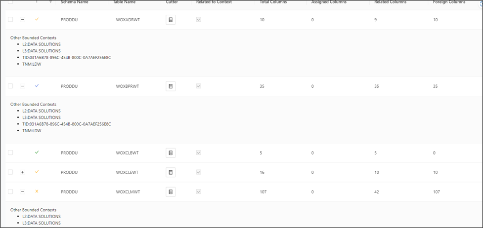
Step 5:
Click the Decompose icon of the associated table.
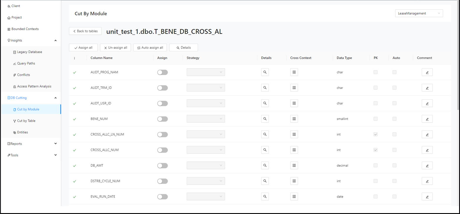
Step 6:
Click Auto Assign All .
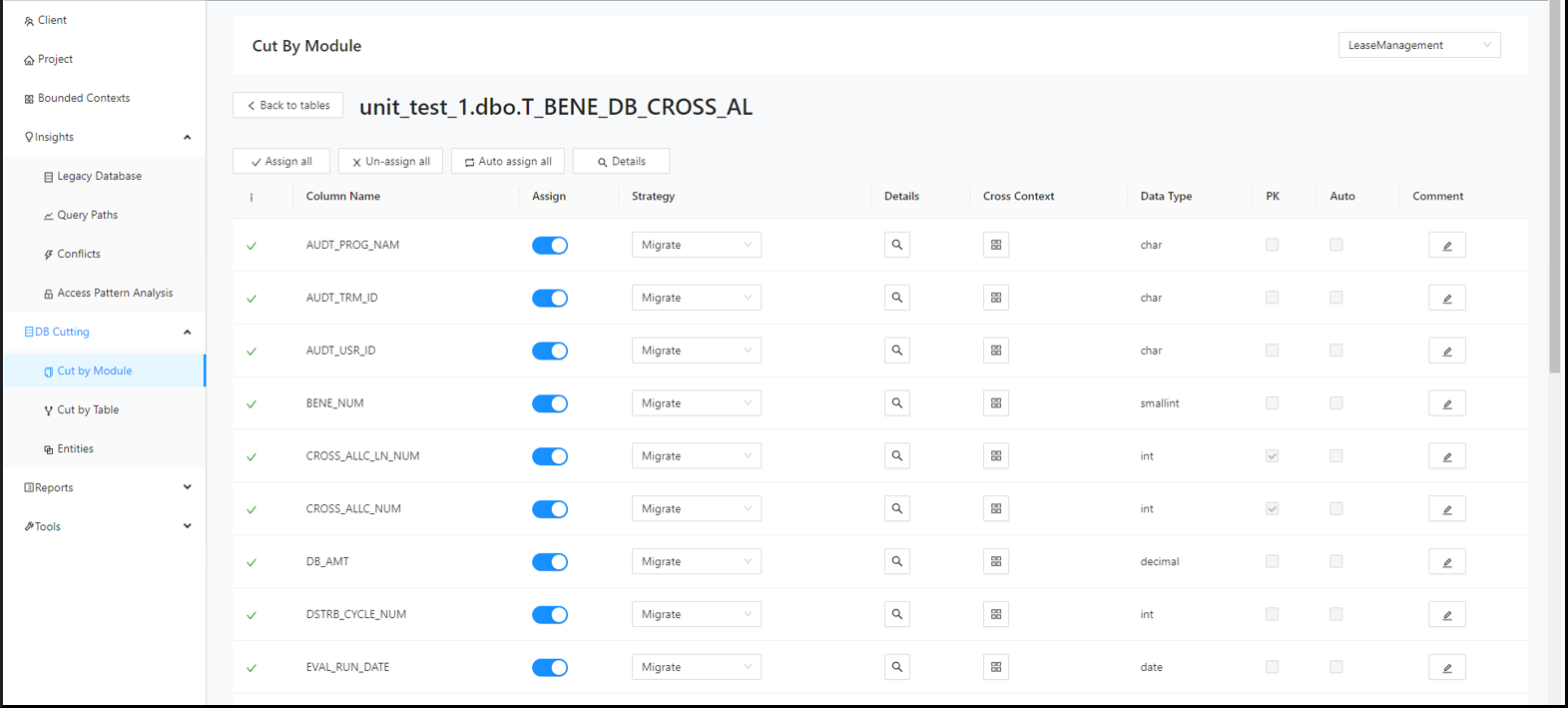
If a column that is part of a join condition is assigned, a warning message will appear.
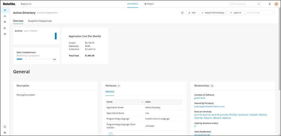
Columns that are part of a join are clearly marked. If you assign a column that belongs to a join, the page notifies you.
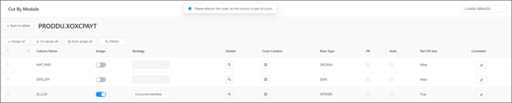
Step 7:
Click Back to Tables .
Step 8:
Click the Decompose icon of the associated table.
Step 9:
Assign the desired column.
Step 10:
Click the corresponding details icon to learn more details about a specific table column, such as referring modules, referring Bounded Contexts and even the actual query code (read/write) used to query the column.
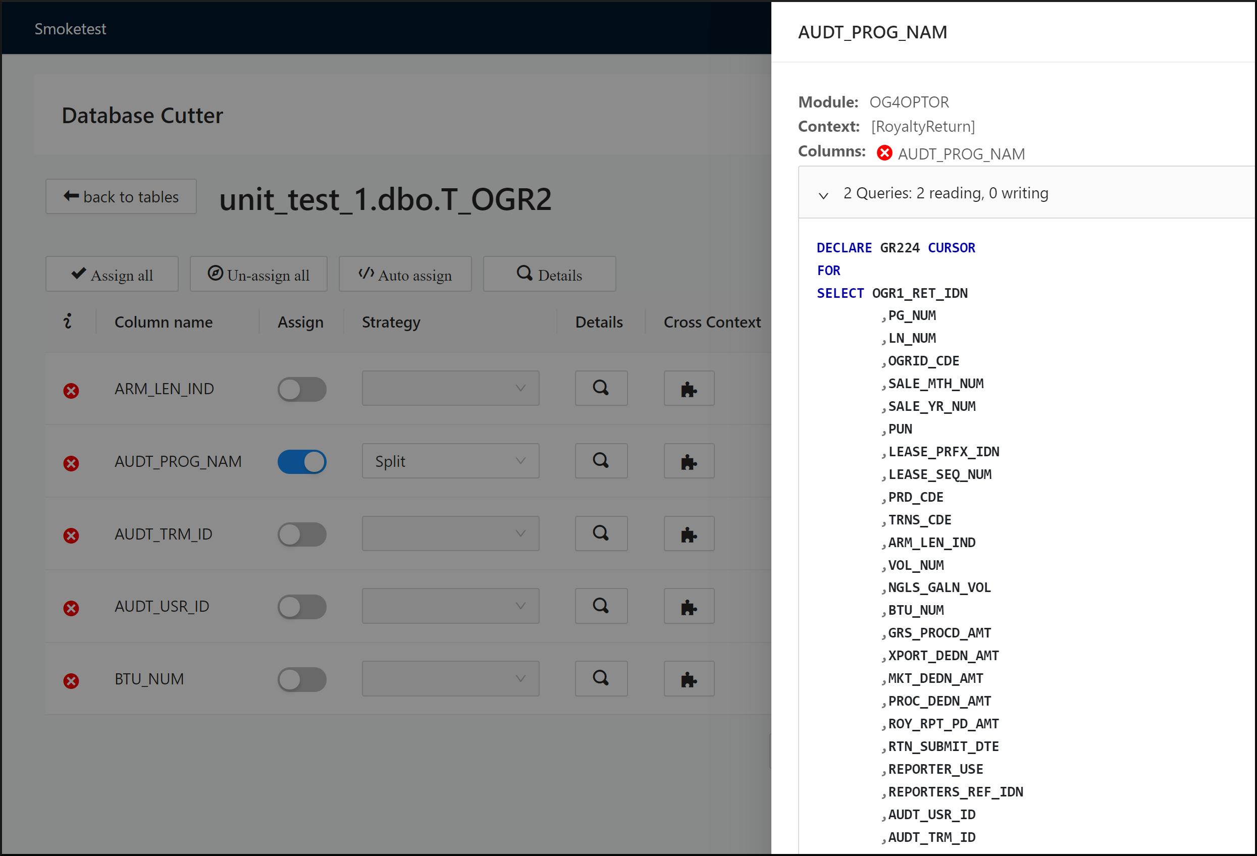
Step 11:
Click the Cross Context puzzle icon. A cross context allows columns/tables to be assigned to multiple bounded contexts. This means that they are not necessarily tied to only one bounded context.
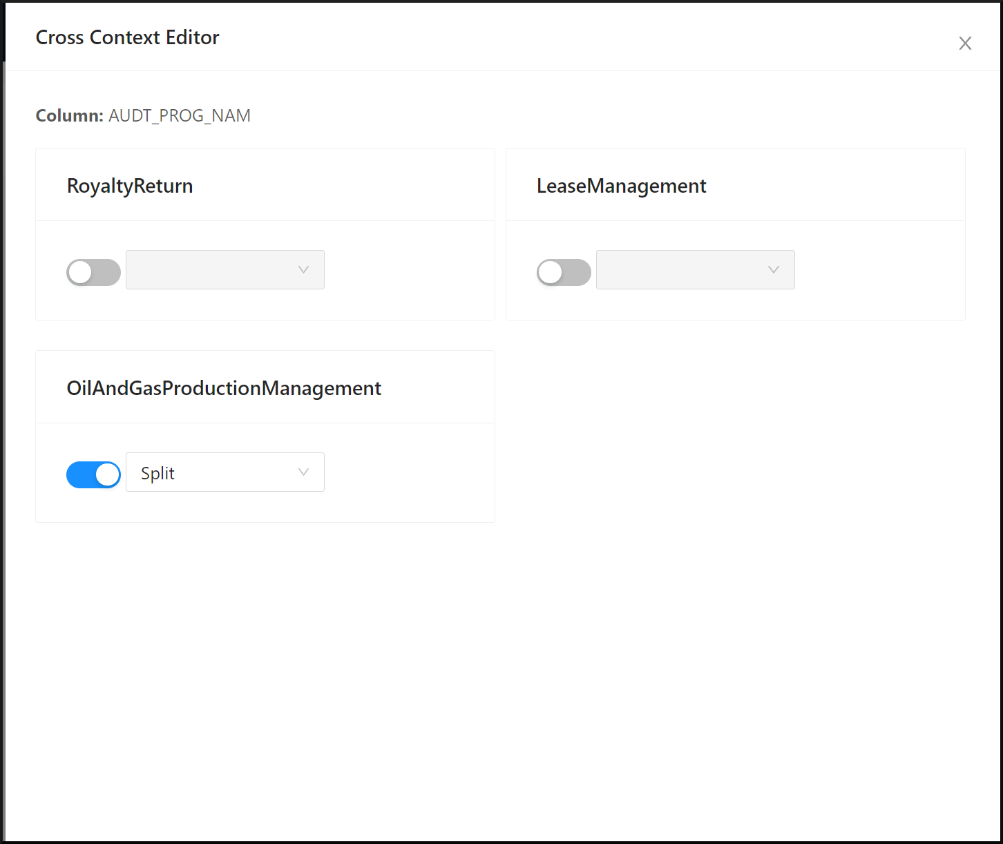
DB Cutting strategies
For cutting a database and designing a suitable target database, it is required to migrate the tables and columns correctly. Decompose provides 5 strategies for cutting a database:
-
Migrate: This is the default strategy when there are no conflicts or if the conflicts can be easily resolved. This means that the column is going to stay as-is in the currently selected bounded context.
-
Split: If a table is part of more than one bounded context, creating a conflict, you can decide which bounded context the table should eventually belong to or split the table's columns across both bounded contexts. In this case, the table would still be part of multiple contexts, but not all columns will be present in all of them. The columns can be split as required. For example, you can have column1/column2 within context1 and column3/column4 within context2.
-
Duplicate: This strategy is used when the column needs to be added to the currently selected bounded context as well as the other bounded contexts where it is present. Changes made to a duplicated context will not reflect on the other. This is the difference between the Duplicate and Replicate strategies.
-
Consume Interface: This strategy can be used when a column is not part of the assigned context and is part of another context which needs to provide an API to access the column. If the same column is present in different bounded contexts then one will be migrate and the other will be consume interface.
-
Replicate: This strategy is similar to the Duplicate strategy, except that changes in one of the replicated contexts will also be reflected in the other.
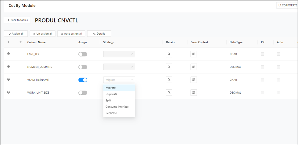
Cut by Table
The Cut by Table feature lets you cut the database based on the available table structure. You can select a table from the full database table list and filter that list by table name.
In the details view of a table, users can select multiple bounded contexts for each column and assign the selected column/context combination according to the modernized database of the context. Additionally, a migration strategy can be selected for each column/context combination.
Bounded contexts can be created and assigned to multiple columns and tables.
To start cutting by table, import the schema, bounded contexts, modules, and queries, and then select the table to cut from the Cut by Table view.
To use the Cut by Table feature, perform the following steps:
Step 1:
In the left navigation panel, select DB Cutting > Cut by Table.
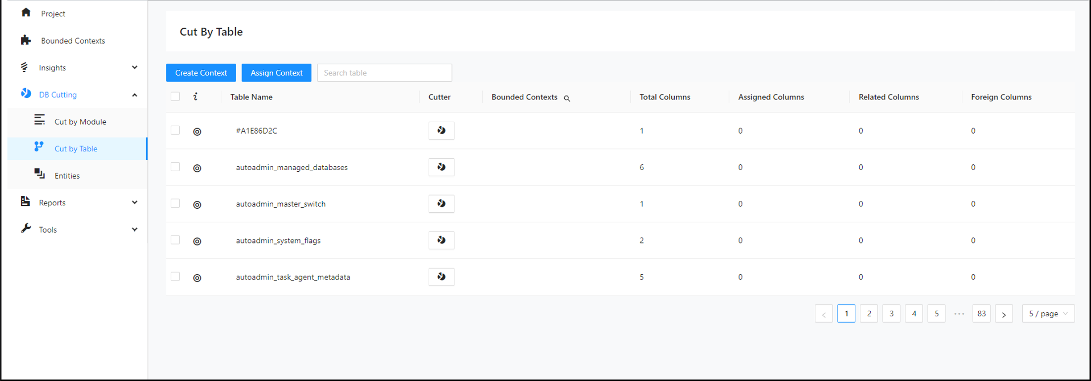
Step 2:
Use the Search bar to find the table you would like to cut.
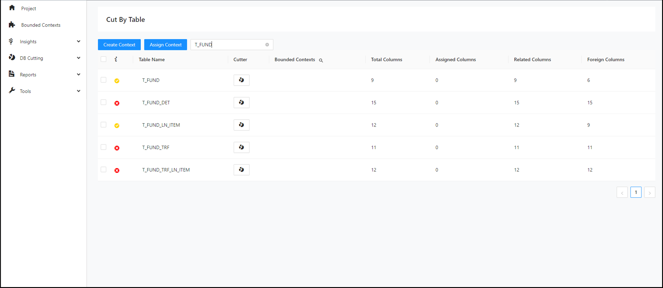
Hovering over the icons beside the tables displays information about all the bounded contexts accessing the table.
Step 3:
Click the Decompose icon next to your selected table.
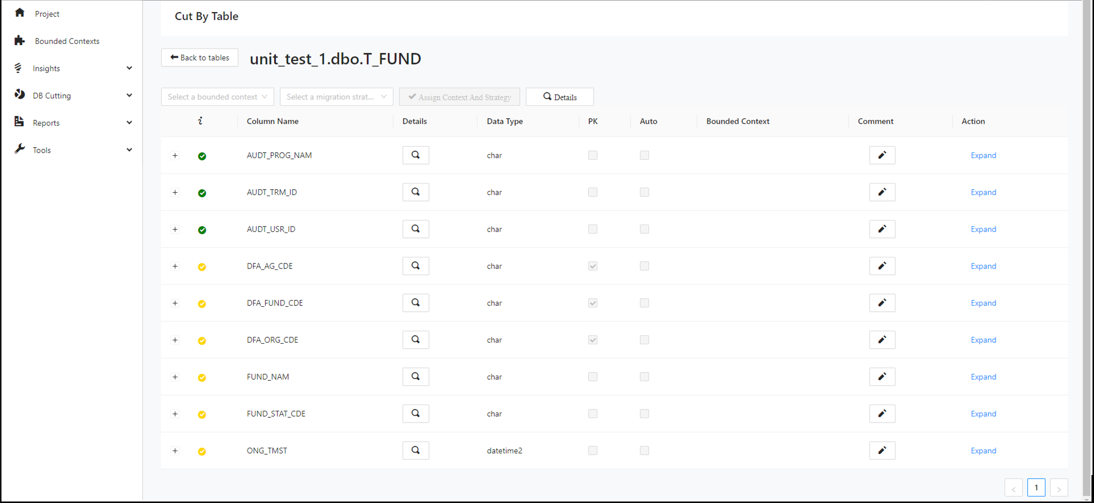
Step 4:
Expand the first column of the table and click Add Relation .
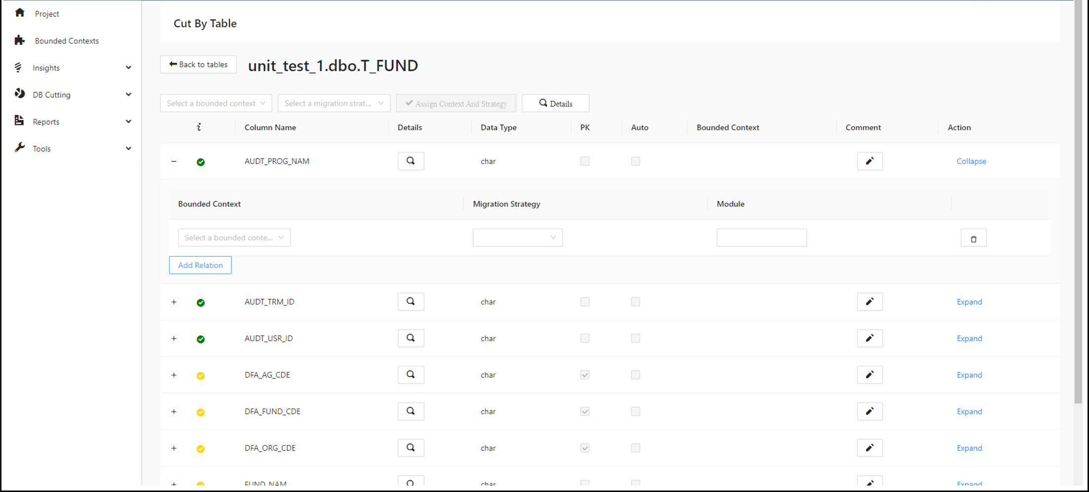
Step 5:
Select the desired bounded context, migration strategy and module.
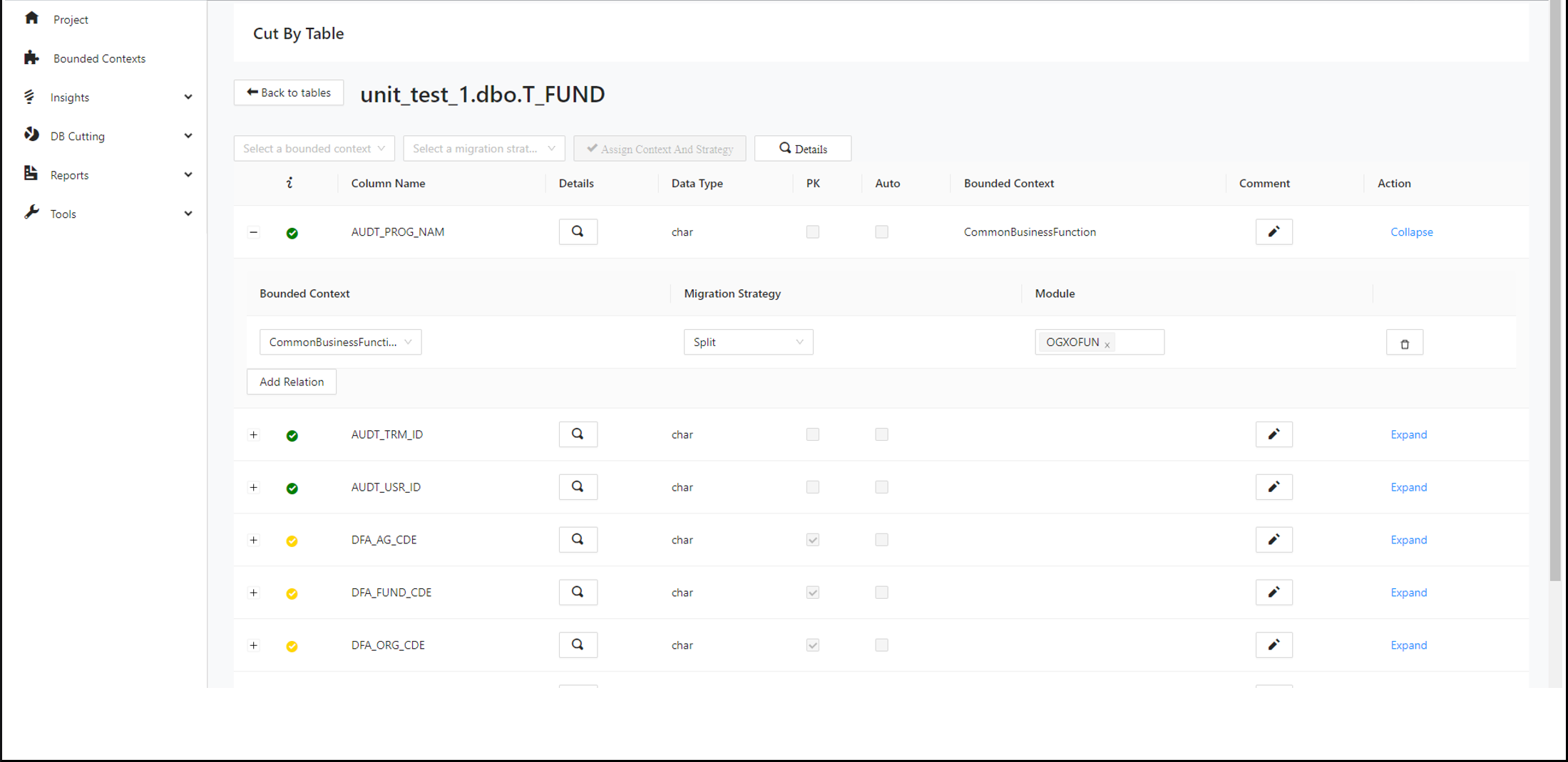
Search for assigned tables and columns
Users can search for the assigned tables and columns on the Cut by Module page.
Step 1:
In the left navigation panel, navigate to Cut By Module and search for the desired table by its bounded context.
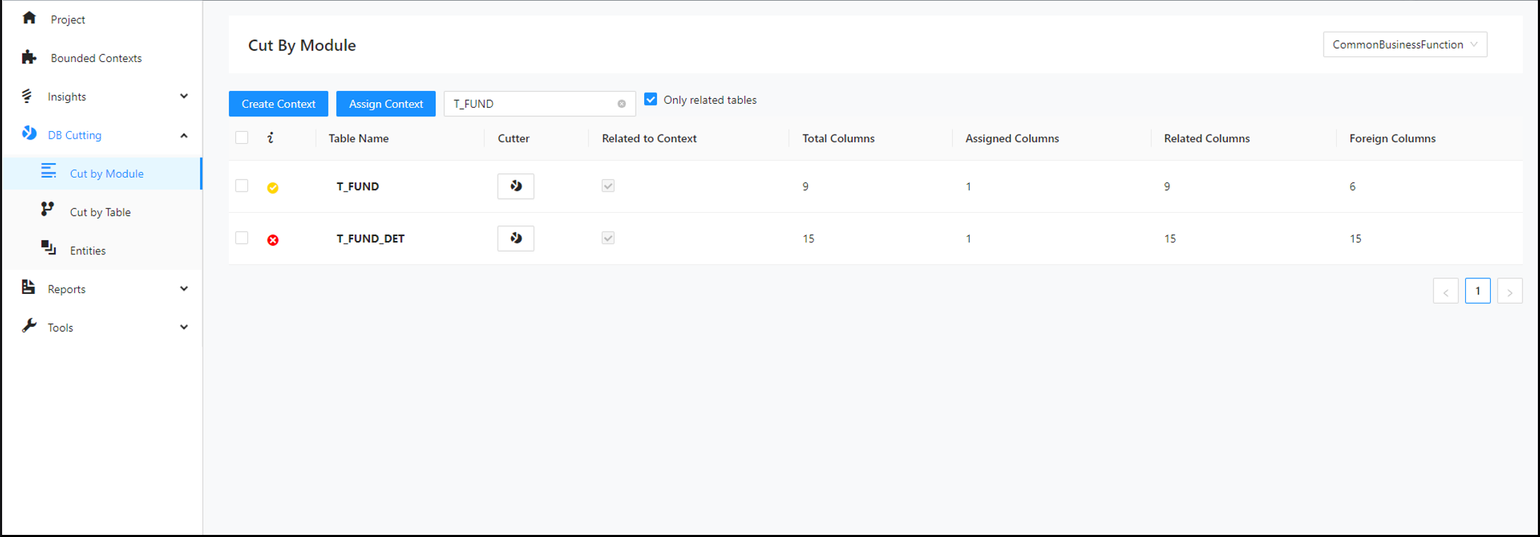
Step 2:
Click the Decompose icon next to your selected table.
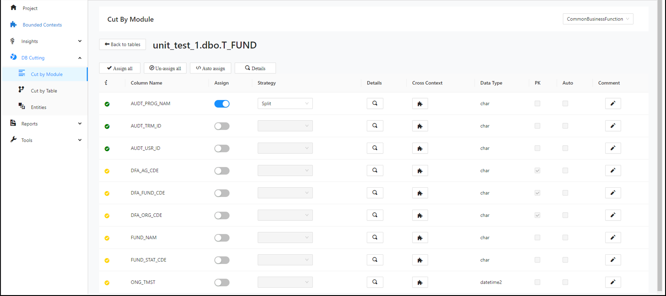
Step 3:
Click Back to tables and select the desired context.
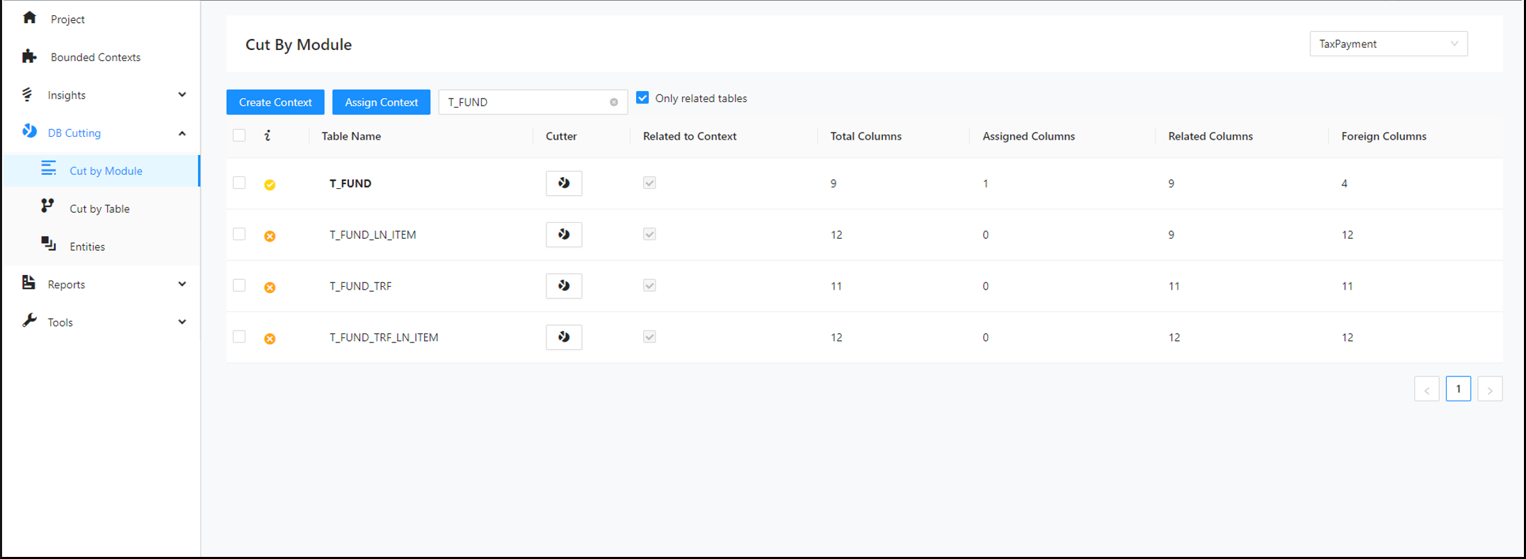
Step 4:
Search for the table you would like to cut and click the Decompose icon next to your selected table.
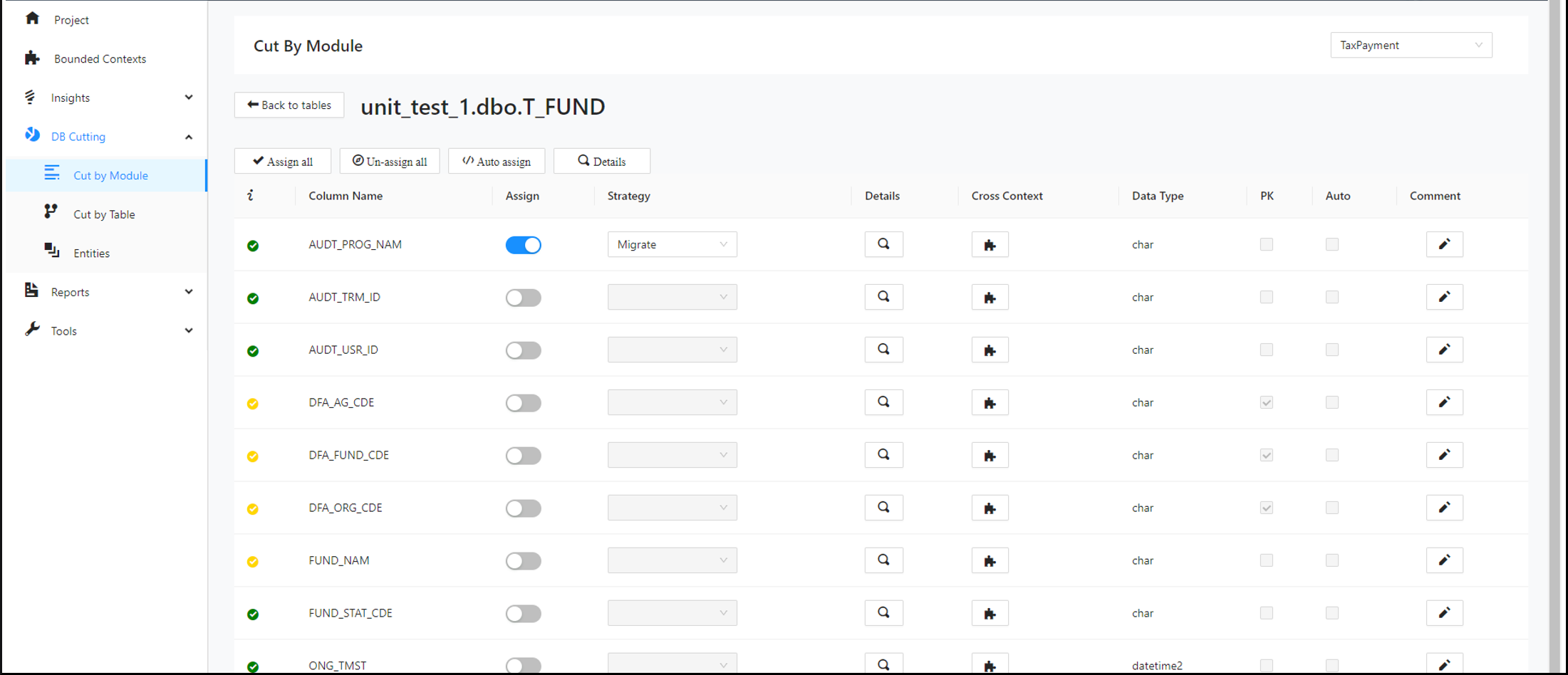
Add relations to all columns of a table simultaneously
Users can add relations to all columns of a table at the same time.
Step 1:
Navigate to the Cut by Table page and search for a table. In the search results, click the Decompose icon. From the dropdowns in the upper part of the page, select a bounded context and the desired migration strategy. Then click Assign Context and Strategy .
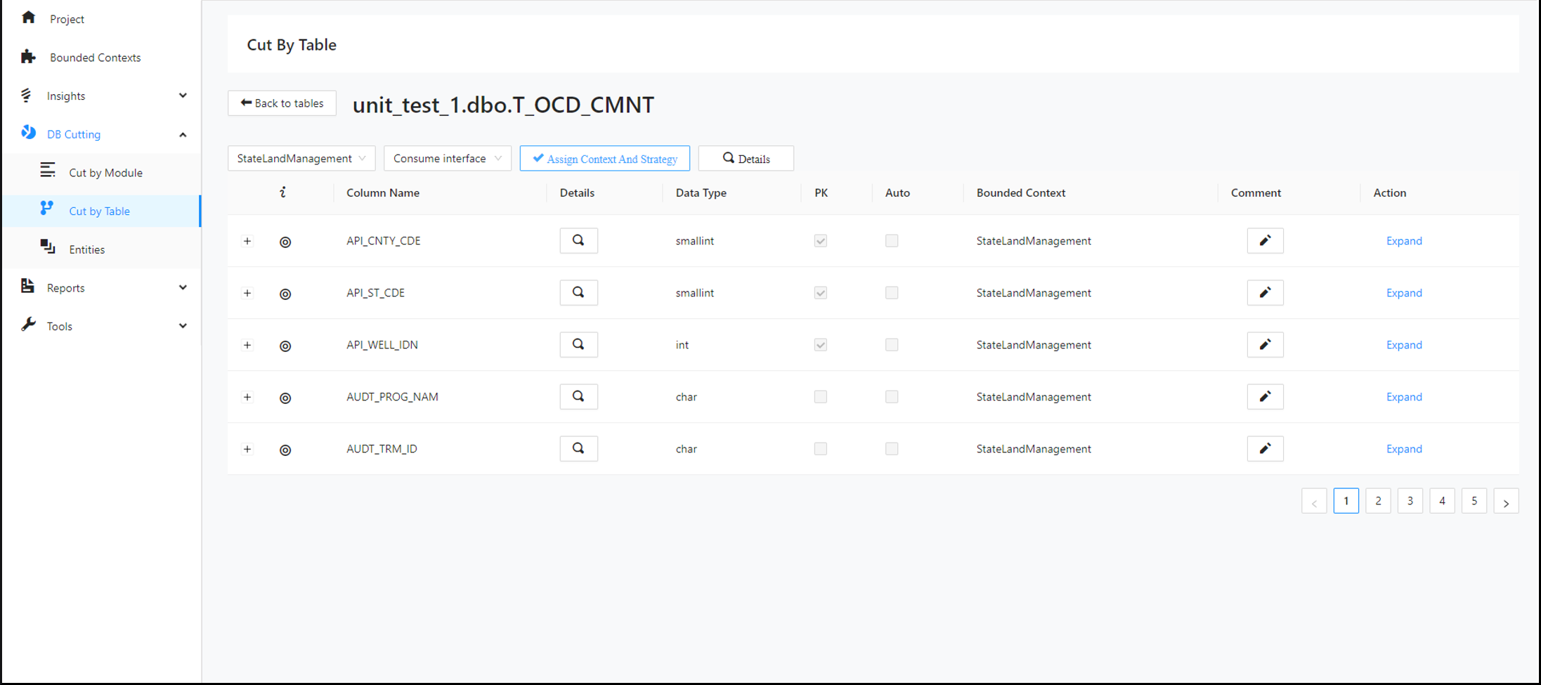
Step 2:
Again, select another bounded context and another desired migration strategy from the dropdowns. Then click Assign Context and Strategy .
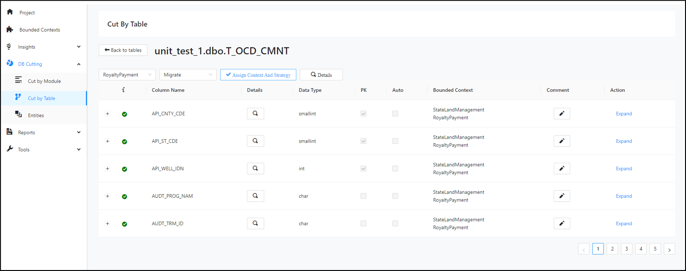
Assign Bounded Contexts to multiple tables simultaneously
Users can assign bounded contexts to multiple tables at once.
Step 1:
Search for a desired table. Select all tables at once by clicking the checkbox in the table header.
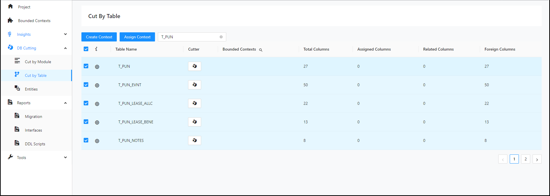
Step 2:
Click Assign Context . From the pop-up menu, select the desired context and migration strategy and click Assign Context and Strategy .
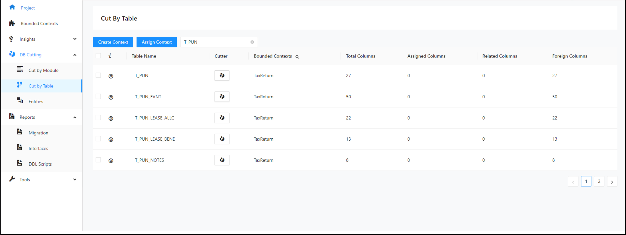
Assign multiple tables simultaneously to a context
You can assign multiple tables at one time to a defined context.
Step 1:
Click Create Context . Set a desired name and click Create .
Step 2:
Search for a desired table and select it. Click Assign Context . From the pop-up menu, select the context you created and click Assign Context and Strategy .
Entities Designer
After you assign columns to a bounded context on the Decompose page, the tool can identify the tables and columns that will become part of the new microservice database for that bounded context. You can then edit the design of the new microservice database, including renaming tables and columns, adding or removing tables, adding relationships, and changing the target database.
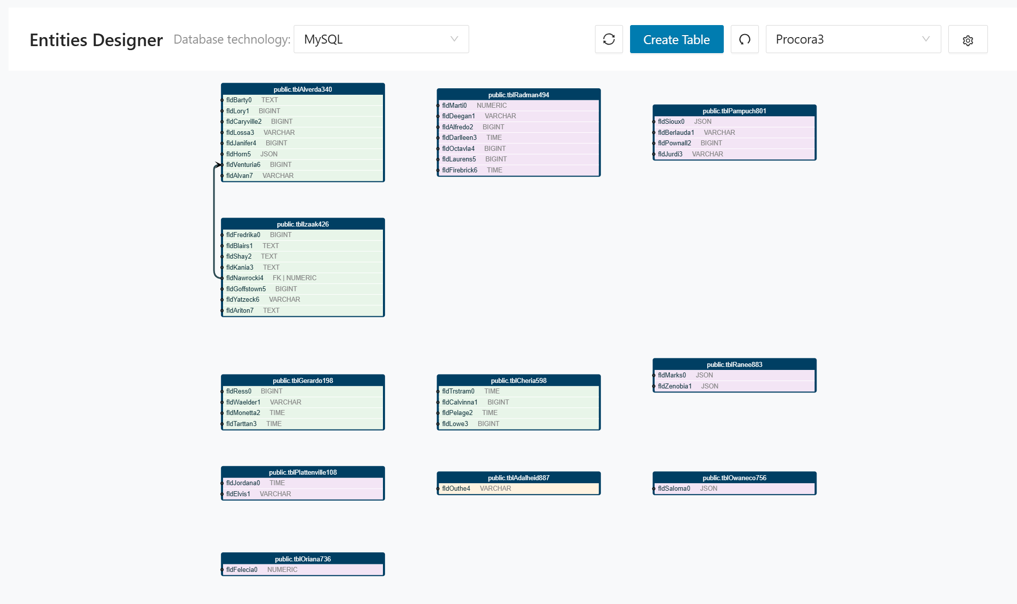
Right-click in the editor area to display the available options. When you are finished, click Save to store your changes in the Decompose database. The next time the Entities Designer opens, it uses the stored database design instead of generating a new diagram from the assigned columns.
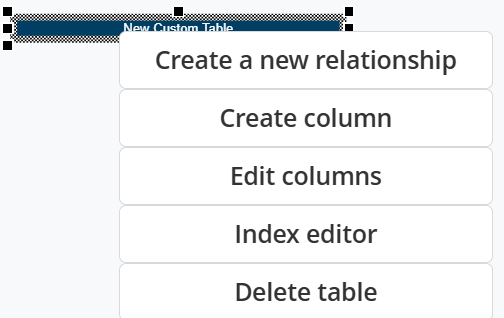
To create a relationship between two databases (entities), click Create New Relationship and complete the form shown below.
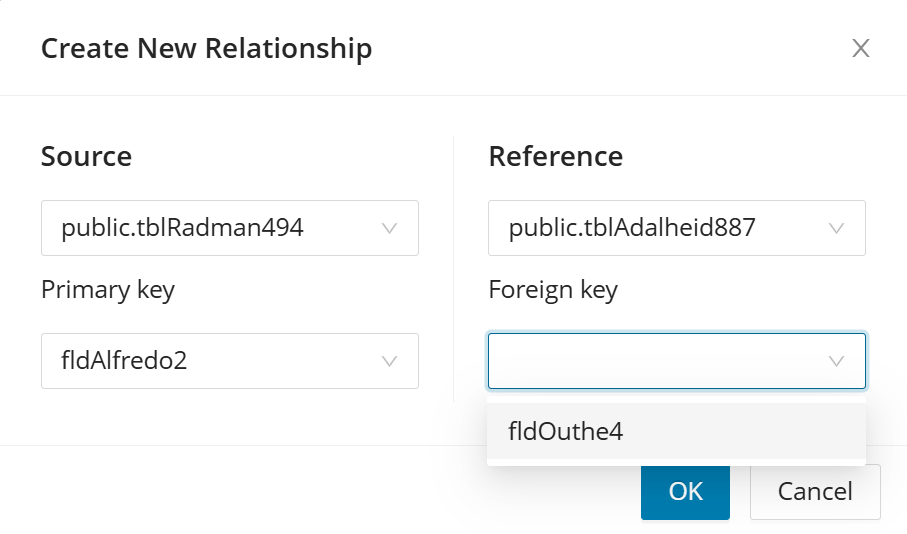
Select the source and target entities (and the fields to join), set the relationship type (for example, one-to-one, one-to-many), then click OK. The tool will add the relationship and visually connect the two entities in the diagram.
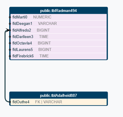
Saving is also necessary to generate the DDL script that can be used to generate the MicroService database.
ER Diagram
The ER Diagram area gives you several visual and tabular ways to inspect the target schema for a bounded context. These views help you review relationships, validate structural details, and prepare downstream implementation artifacts. Use the mode that best matches whether you are discussing the design, editing metadata, or exporting SQL artifacts.
Entity Relationship Diagram
Tables are rendered as “cards” showing table name plus key columns/attributes (and typically relationships when enabled).
Best for: human-friendly schema review, discussing structure with stakeholders, and spotting missing/duplicated entities or attributes.
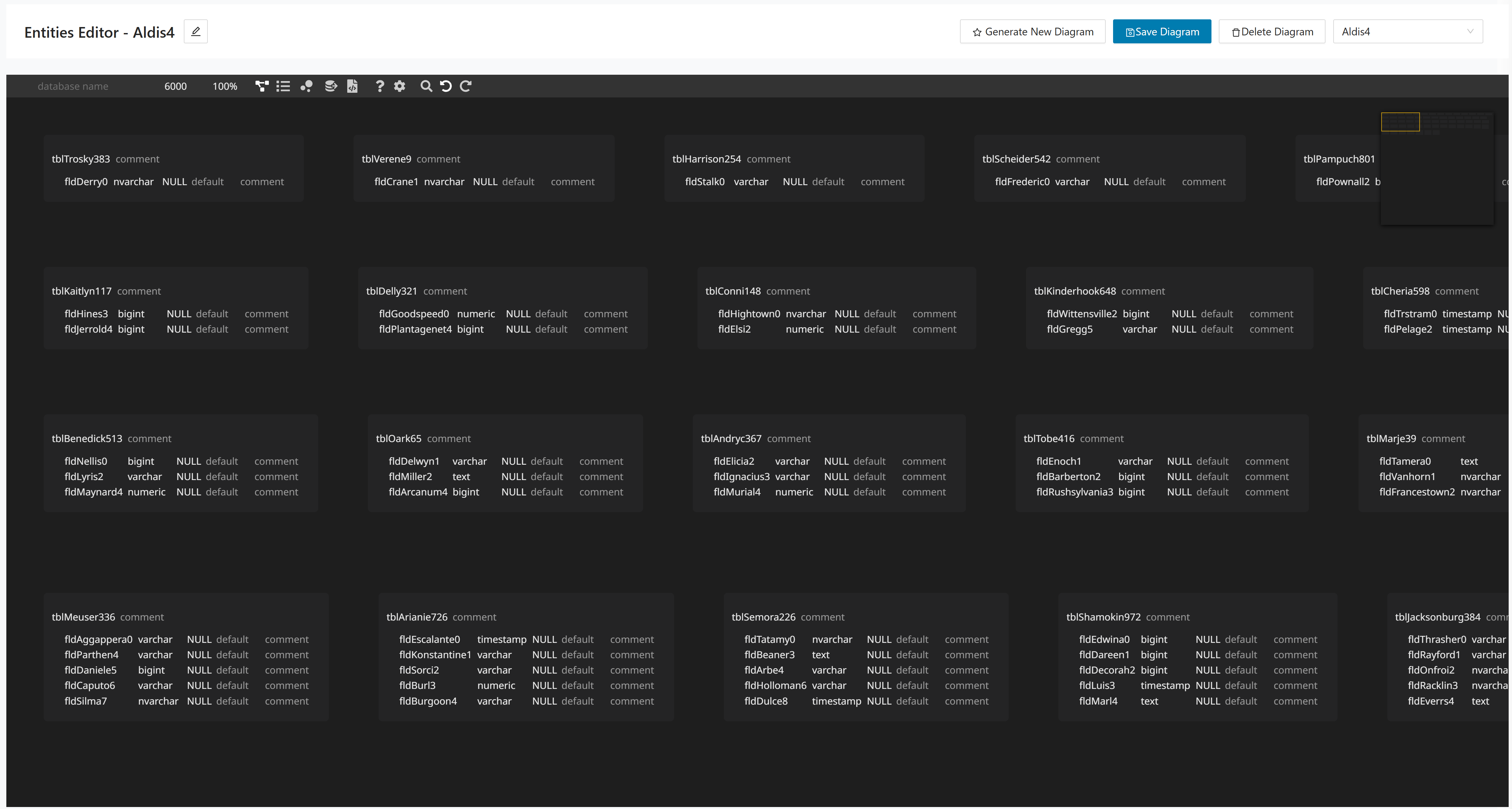
Grid
A spreadsheet-like grid listing Table Name, Table Comment, column/field Name, DataType, and options/metadata.
Best for: bulk edits (rename fields, change data types, update comments), sorting/filtering, and fast QA of column definitions.
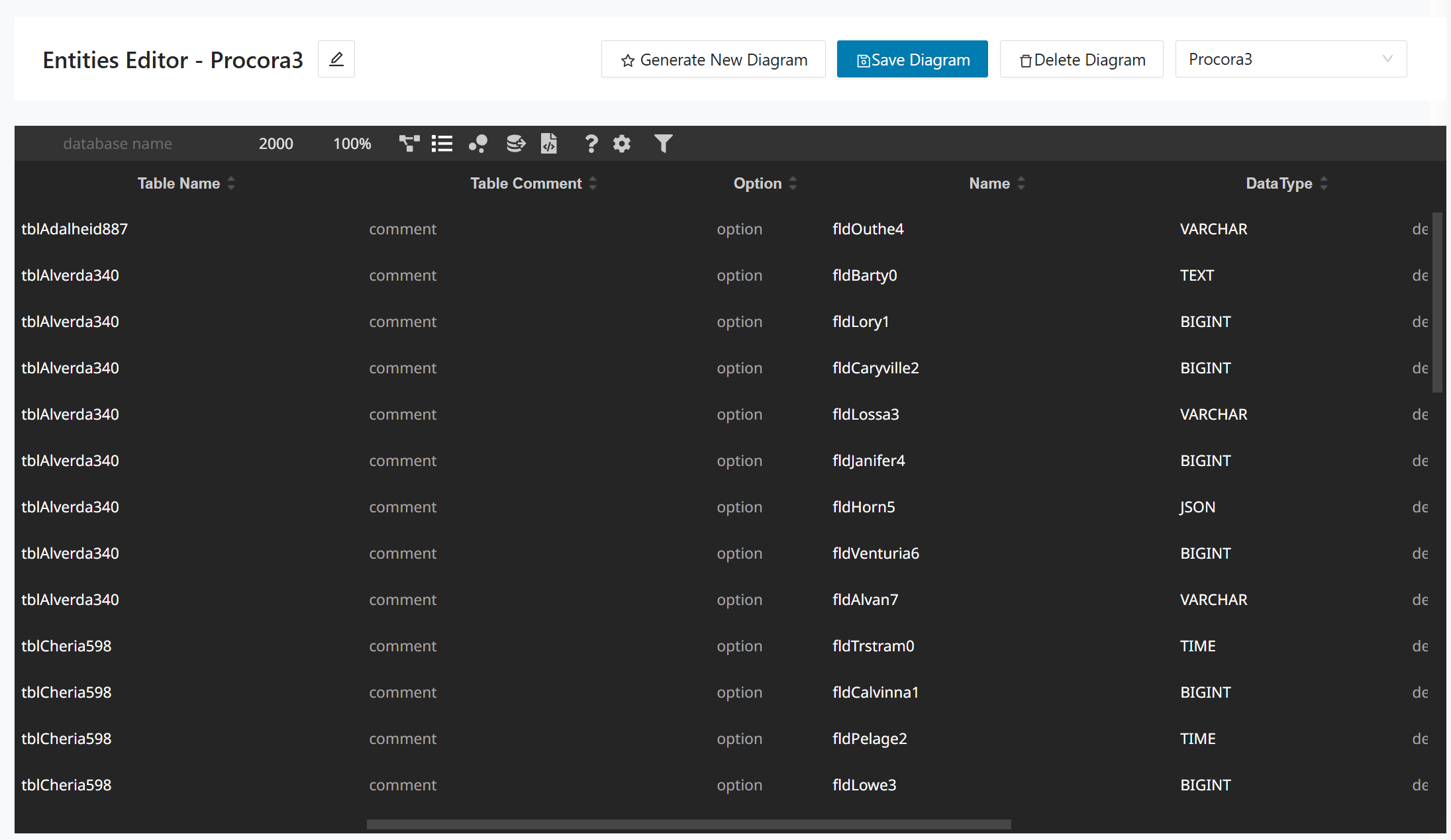
Visualization
A force-directed graph where nodes and links show connectivity (commonly tables and their relationships; sometimes columns/keys as leaf nodes).
Best for: understanding clusters, highly-connected “hub” entities, and the overall complexity/shape of the bounded context.
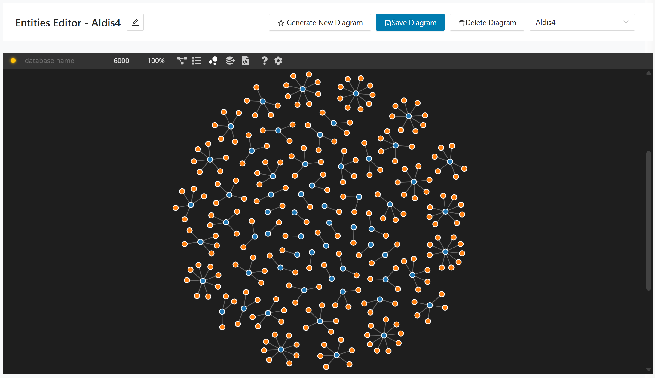
SQL DDL
Generates CREATE TABLE ... statements with columns, data types, and constraints (for example, NULL).
Best for: applying changes to a database, sharing with DBAs, and validating that the modeled schema maps cleanly to SQL.
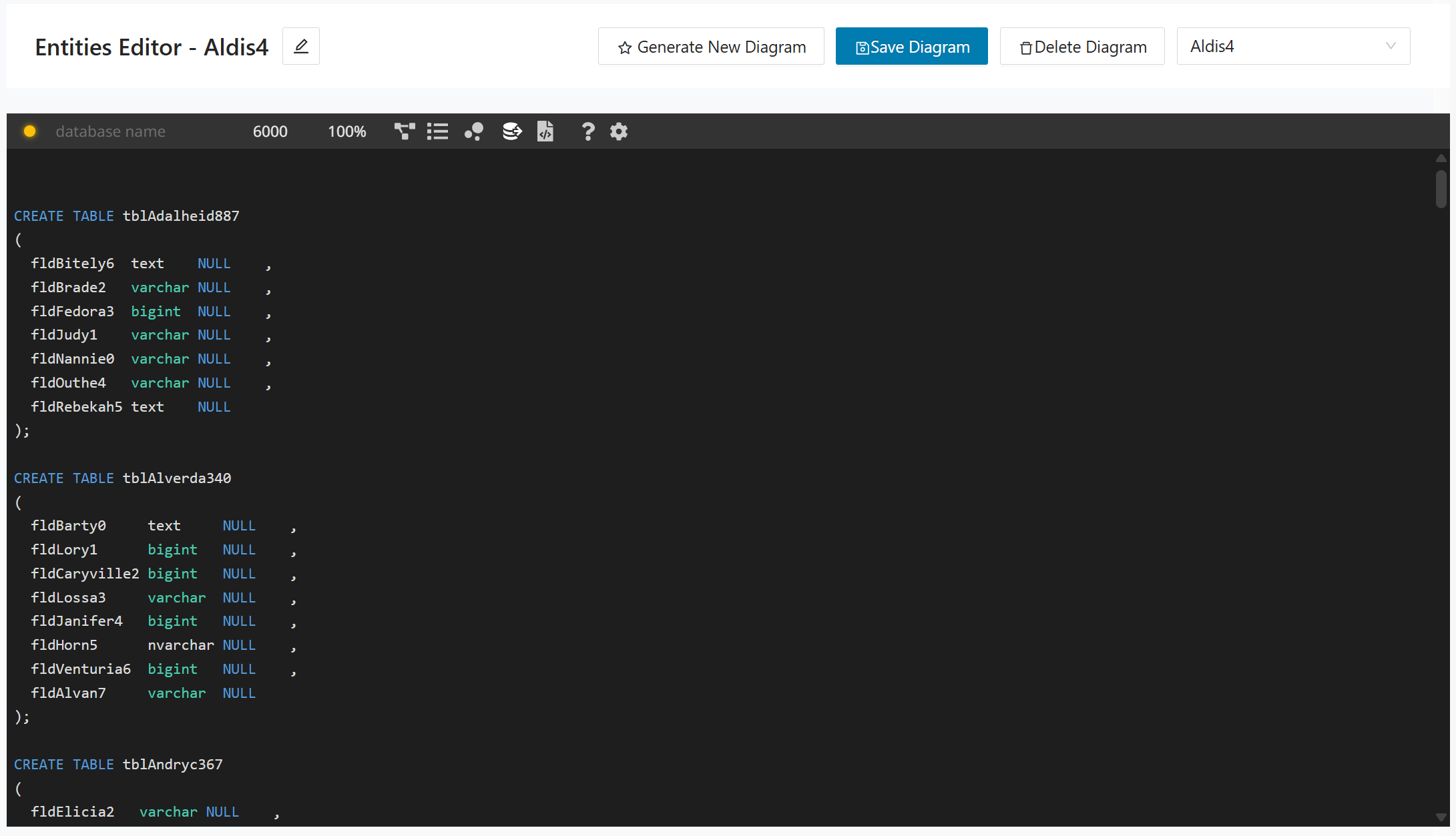
Generator Code
Shows table/entity definitions in a code/DSL format (for example, type Tbl... { field: Type }).
Best for: quick copy/paste into source control, reviewing names/types at speed, and generating downstream artifacts from a single definition.
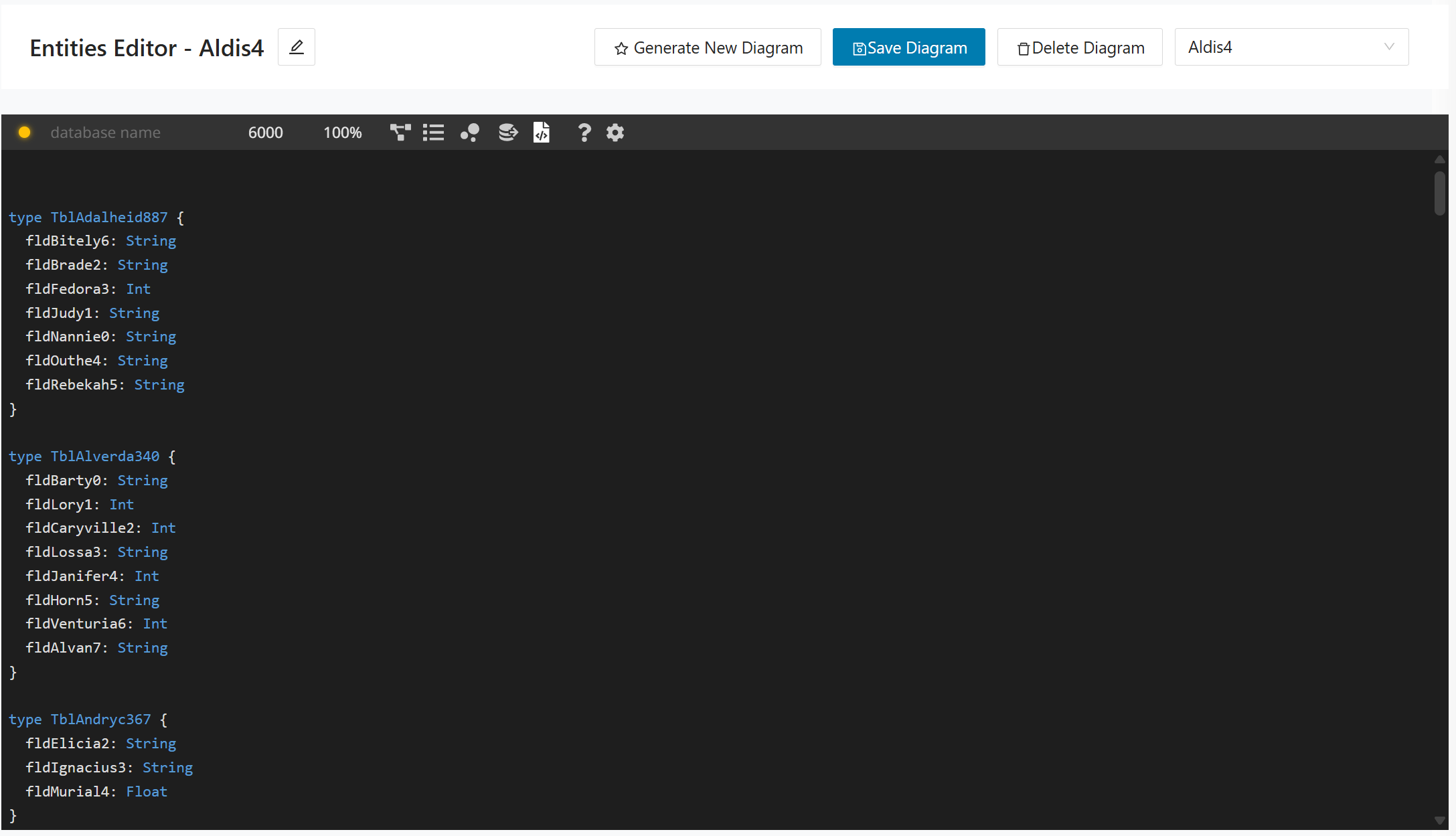
DDL Generator
The DDL Generator creates SQL DDL statements for the selected bounded context based on the database design saved in the Entities Designer. Use this page when you want to review the generated schema, copy it for implementation work, or export the generated DDL for multiple target dialects.
If no entities have been saved for the selected bounded context, the page shows a No DDL Generated message. In that case, define the required tables in Entities Designer, save the model, and then generate the DDL again.
To generate DDL, perform the following steps:
Step 1:
In the left navigation panel, select DB Cutting > DDL Generator.
Step 2:
Select the bounded context whose target schema you want to generate.
Step 3:
Select the target database dialect, for example, MySQL.
Step 4:
Click Generate DDL to generate the script for the selected dialect, or click Generate All Dialects to generate all supported dialect variants.
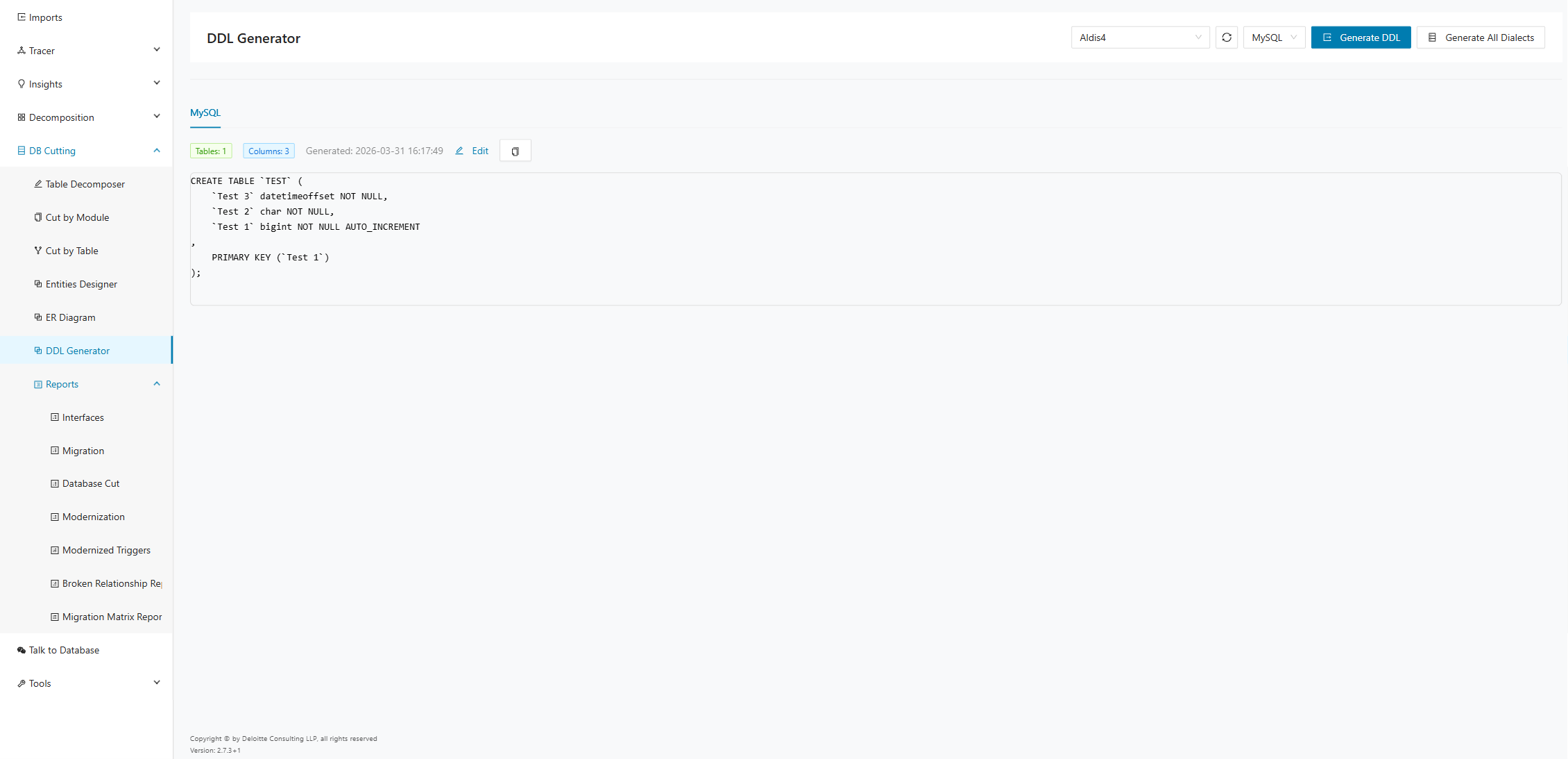
After generation, the page displays the generated dialect in a tab, together with the number of tables and columns included in the script and the generation timestamp. Use Edit to adjust the generated DDL before copying it, or use the copy action to copy the SQL text to the clipboard.
Reports
Use the Reports tab to create and run reports on migrations, interfaces, DDL-related outputs, and cross-context dependencies. The available reports include Interfaces, Migration, Database Cut, Modernization, Modernized Triggers, Broken Relationship Report, and Migration Matrix Report.
Interfaces
The interface report shows which bounded contexts provide interfaces to data that has been migrated to their microservice database. It also shows which other contexts are consuming these interfaces. You can download the report data as a CSV file for automated use in other tools. It shows the necessary connections between microservices, that is, if one microservice holds data that another requires, there must be an interface between them.
The API team (developers) needs this report to provide the interfaces. Run it at least once per microservice.
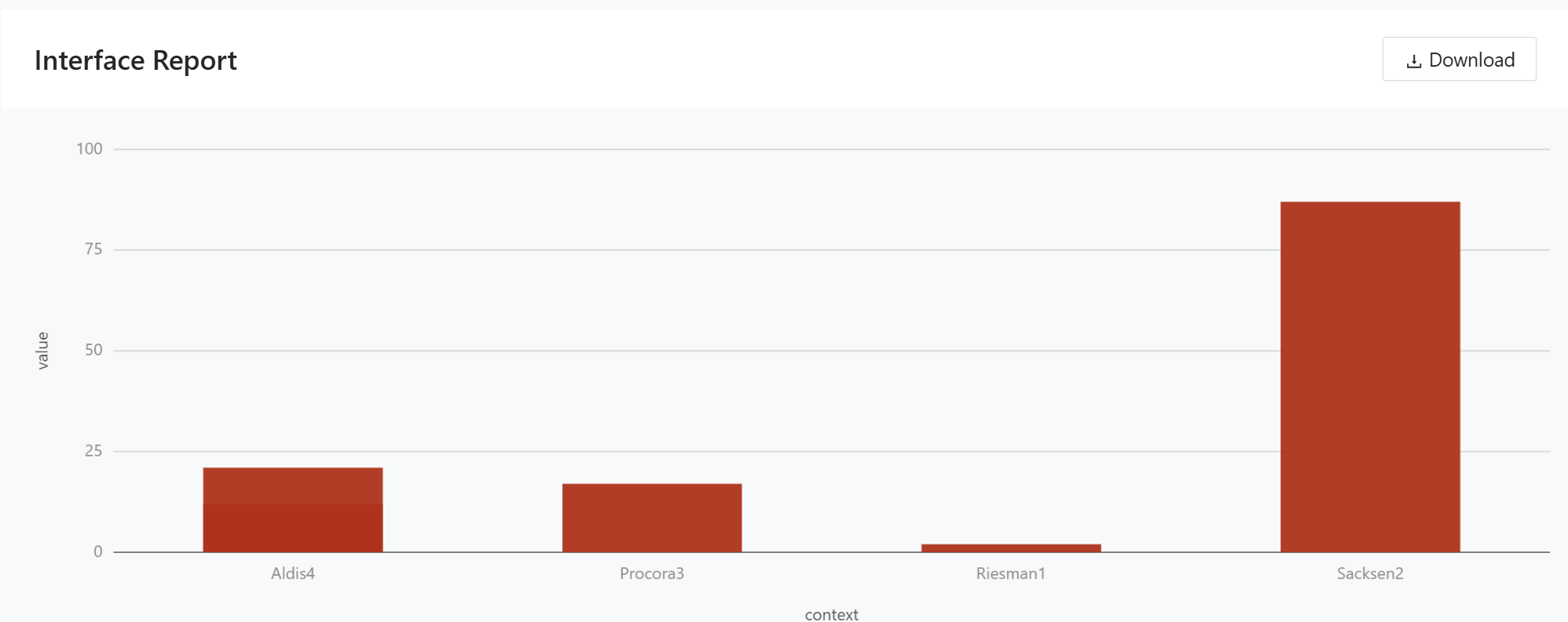
The chart shows the number of tables per bounded context that use the Consume Interface strategy when cutting a module.
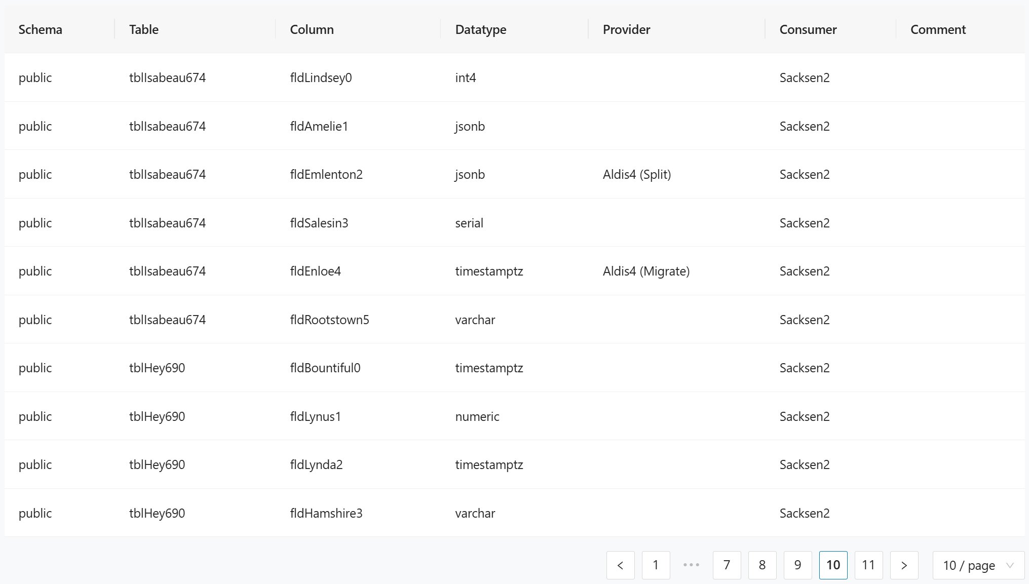
The table lists each interface relationship at the column level:
- Schema identifies the database schema.
- Table identifies the source table.
- Column identifies the source column within the table.
- Datatype shows the column's data type.
- Provider identifies the bounded context that owns the data and its assigned migration strategy (for example, Split or Migrate).
- Consumer identifies the bounded context consuming the interface.
- Comment provides optional notes.
Migration
The migration report shows which data is migrated from specific tables and columns and which bounded context they are associated with. Use the data from this report to jump-start an ETL implementation. You can download it as a CSV file for automated use in other tools.
The graph view of the Migration Report for a selected bounded context. The bounded context node connects through a central API node to all associated database tables, each displayed with their column names and data types. The header provides navigation between bounded contexts, along with Download and Assess Export options.
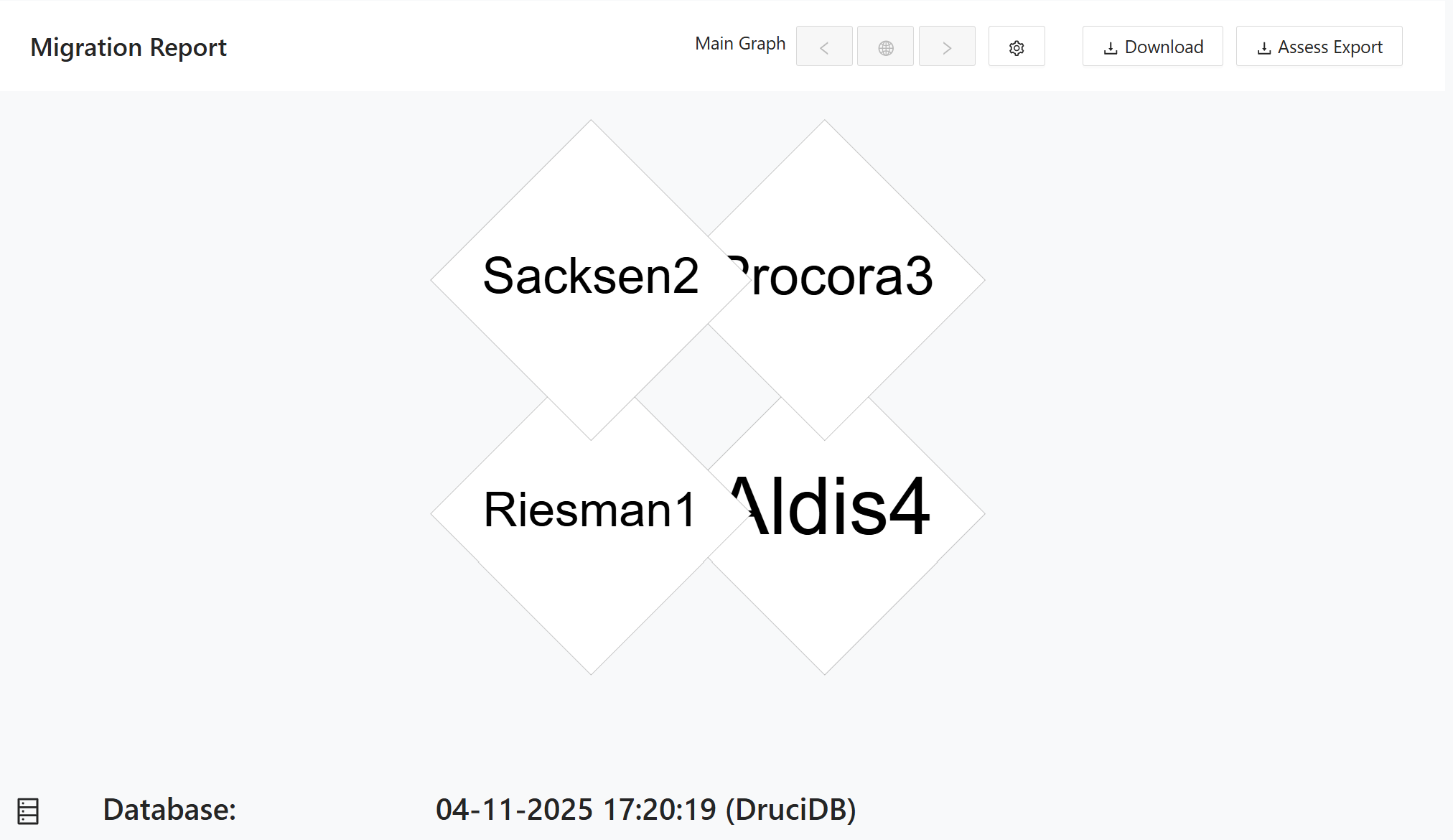
The main graph view of the Migration Report showing all bounded contexts as diamond-shaped nodes. Each node represents a distinct bounded context in the migration. The database name and import timestamp are displayed at the bottom of the page.
Click the
settings icon to customize the graph's display style.
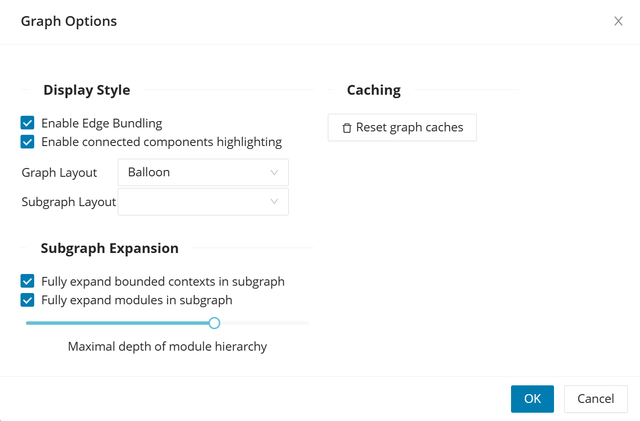
Click a bounded context to expand its details, showing the tables and columns associated with that context along with their assigned migration strategies.
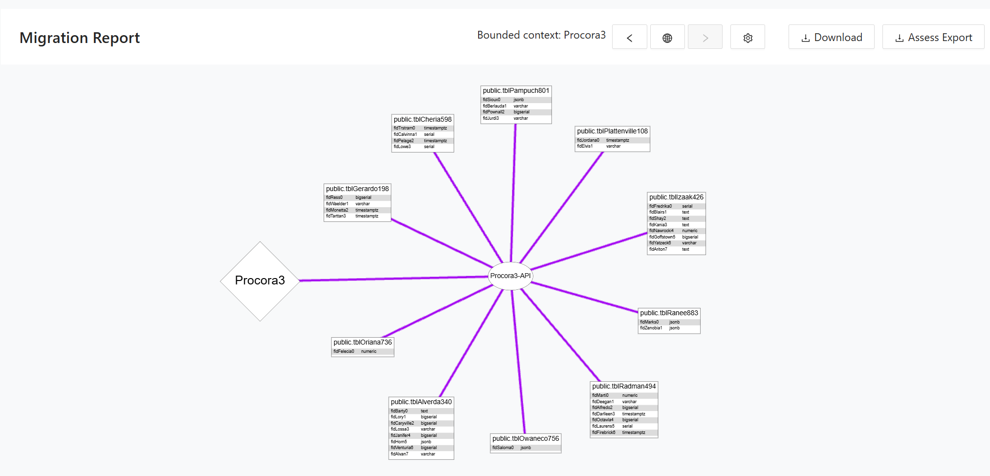
This is another example of a bounded context expanded.
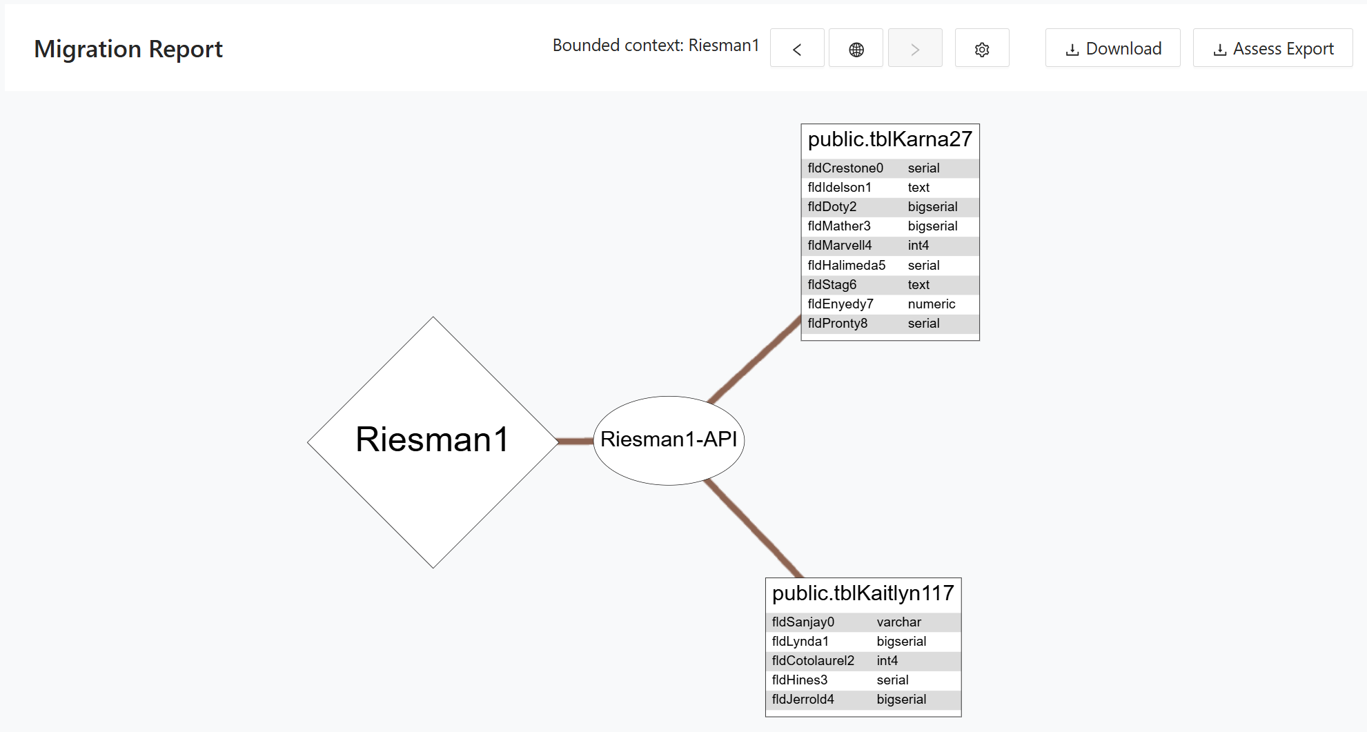
The tabular view of the Migration Report listing each migration entry at the column level. The table contains the following columns:
- Bounded Context identifies the bounded context to which the column is assigned.
- Table identifies the source table containing the column.
- Column identifies the specific column being migrated.
- Strategy identifies the migration strategy assigned to the column (for example, Split or Migrate).
- Comment provides optional notes for the entry.
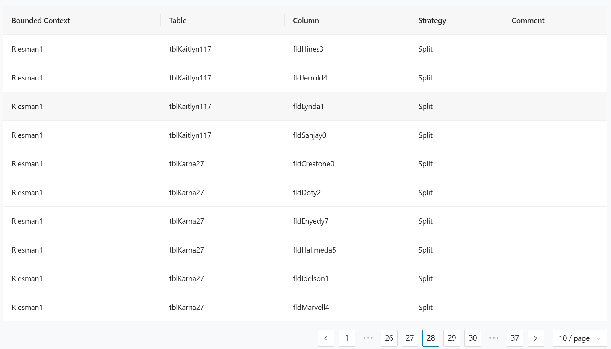
Assess Export
Decompose lets you export the database to import it into Assess. The general workflow is to first import the database schema and then the CSV file with the bounded contexts, modules, and queries.
Then navigate to Reports -> Migration and click Assess Export . This downloads an Excel file containing an overview of the database.
Here's an example of an exported xlsx file:
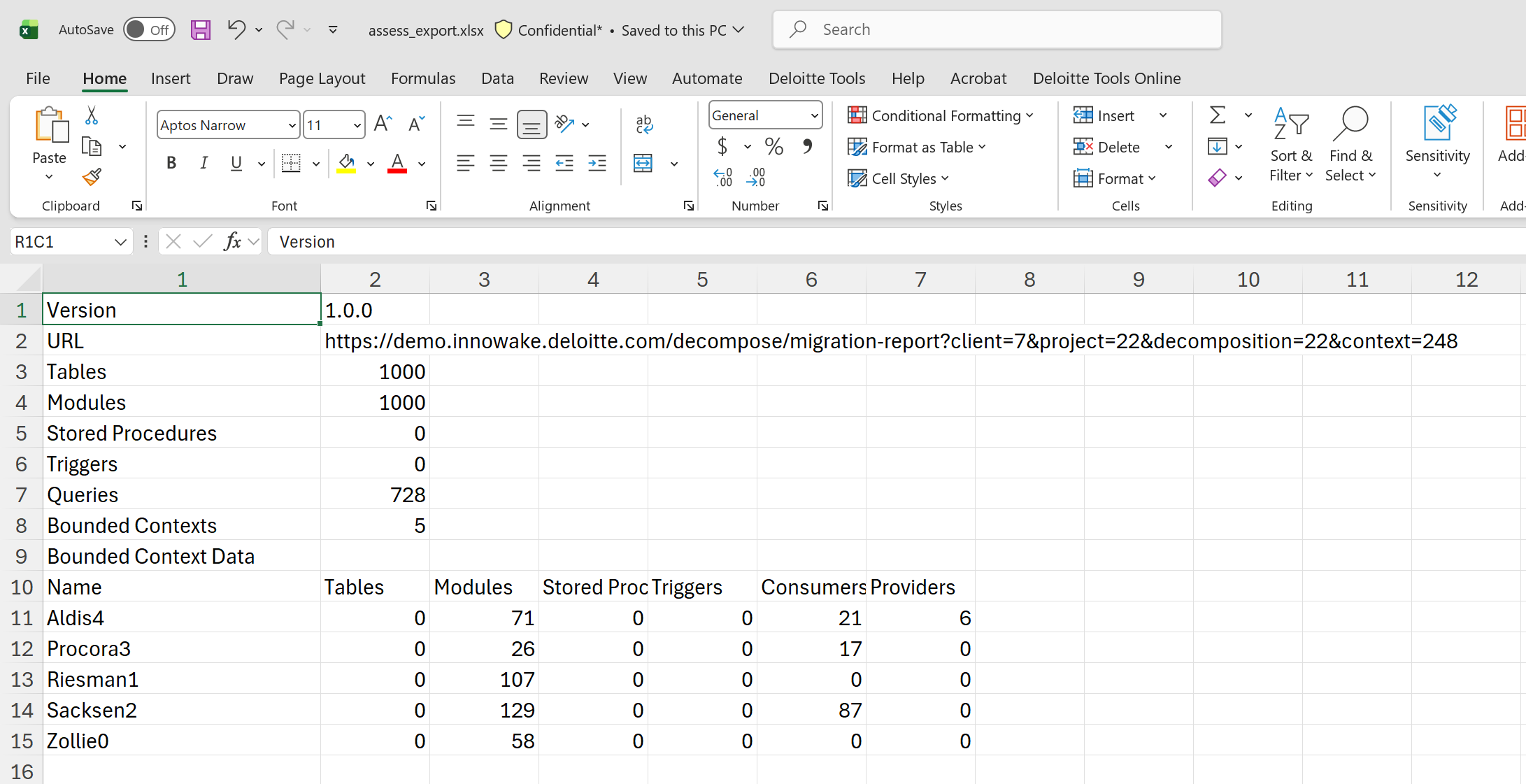
Database Cut
The Database Cut report lists all columns assigned across bounded contexts at the column level. All columns are sortable and can be filtered to narrow down results. The table contains the following columns:
- Bounded Context identifies the bounded context to which the column is assigned.
- Database identifies the source database.
- Schema identifies the database schema.
- Table identifies the source table containing the column.
- Column identifies the specific column included in the cut.
- Strategy identifies the migration strategy assigned to the column (for example, Migrate or Split).
- Reads indicates whether the column is read by the bounded context.
- Writes indicates whether the column is written by the bounded context.
- Comment provides optional notes for the entry.
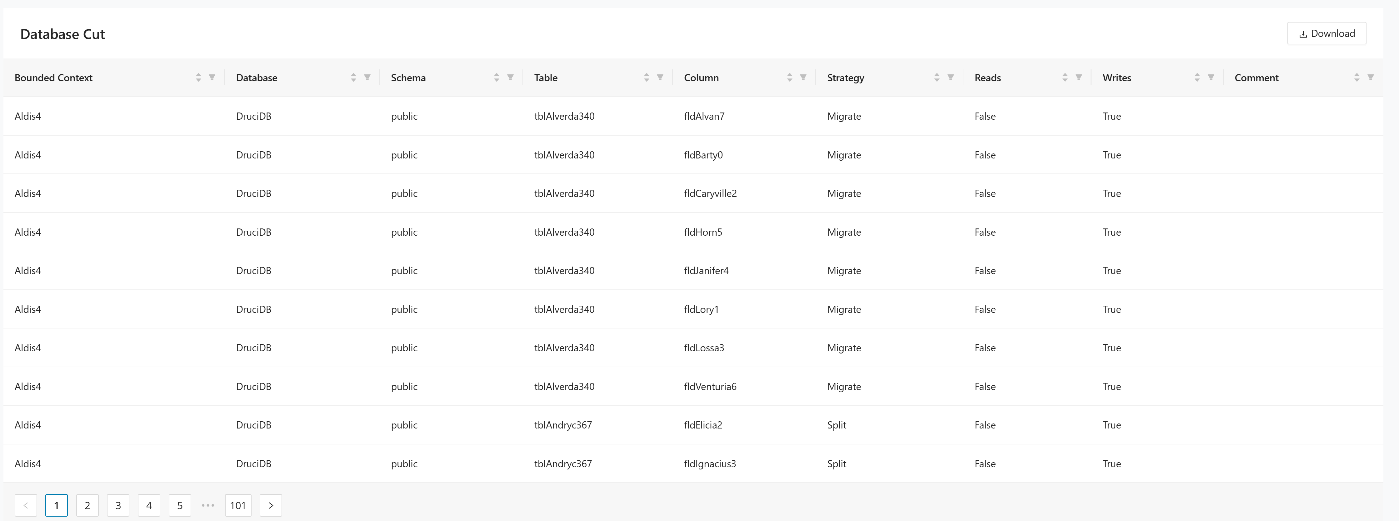
Click Download to export the current table view as a CSV file for use in external tools or further analysis.
Modernization Report
The Modernization Report is populated with the tables and columns defined in the Entities Designer. It provides a side-by-side comparison of the modernized database structure against the legacy database at the column level, showing how each column maps from the legacy system to the new microservice database. All columns are sortable and can be filtered. Click Download to export the report as a CSV file.
The table contains the following columns:
- Bounded Context identifies the bounded context to which the column belongs.
- Database identifies the target database for the modernized structure.
- Table identifies the modernized table name.
- Column identifies the modernized column name.
- Column Type identifies the data type of the modernized column.
- Legacy Table identifies the corresponding table in the legacy database.
- Legacy Column identifies the corresponding column in the legacy database.
- Legacy Column Type identifies the data type of the legacy column.
- Strategy identifies the migration strategy assigned to the column (for example, Migrate or Split).
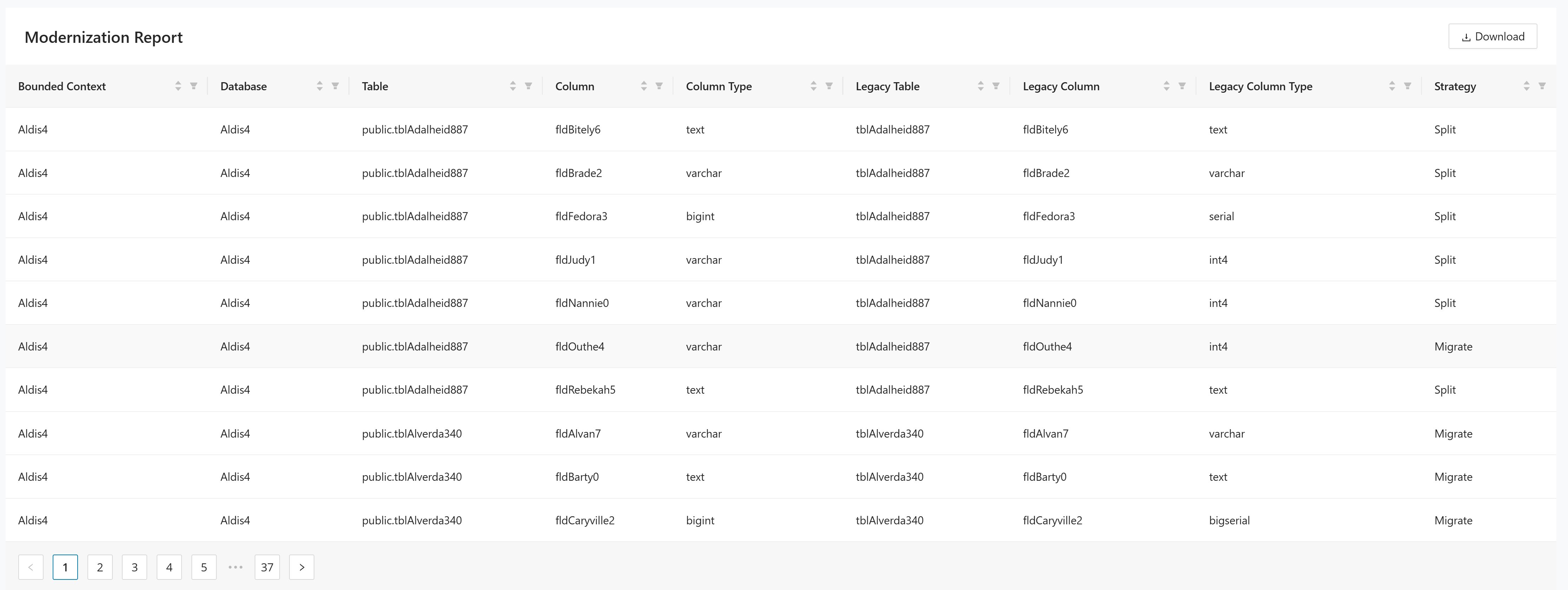
Click Download to export the current table view as a CSV file for use in external tools or further analysis.
Modernized Triggers report
The Modernized Triggers report lists trigger definitions that are associated with the modernized database design across the current project. Use this report to review whether trigger logic has been carried forward into the target schema and to identify missing trigger definitions before implementation.
The table contains the following columns:
- Bounded Context identifies the bounded context that owns the modernized trigger.
- Database identifies the target database that contains the trigger.
- Schema identifies the database schema.
- Table identifies the source or legacy table related to the trigger.
- Modernized Table identifies the target table in the modernized design.
- Trigger Name identifies the trigger.
- Trigger Event identifies the database event that fires the trigger.
- Event Timing identifies when the trigger executes, for example, before or after the event.
- Statement shows the trigger statement or expression.
To populate the Modernized Triggers report
Make sure that the project contains imported legacy trigger metadata together with a saved modernized database design. In practice, this usually means the following:
To populate the Modernized Triggers report,
1. Import the legacy schema in Imports > Schema Upload. Trigger metadata comes from the schema import, and there is no separate trigger-import page.
2. Import the related modules and queries in Imports > Modules and Queries. Decompose imports trigger activity together with the module/query data used for analysis.
3. Assign the affected legacy tables and columns to bounded contexts in Cut by Module or Cut by Table.
4. In Entities Designer, create or update the target database design for the bounded context and save it. The report depends on the saved modernized database design.
5. Open DB Cutting > Reports > Modernized Triggers to verify the generated rows and export them if needed.
After these prerequisites are met, the report shows one row per trigger associated with the modernized design.
Example:
| Bounded Context | Database | Schema | Table | Modernized Table | Trigger Name | Trigger Event | Event Timing | Statement |
|---|---|---|---|---|---|---|---|---|
| Order Management | order_service_db | dbo | Orders | order_header | trg_orders_audit | UPDATE | AFTER | INSERT INTO order_audit (order_id, changed_at) VALUES (NEW.id, CURRENT_TIMESTAMP); |
If no trigger definitions are available for the current project, the report displays an empty state.
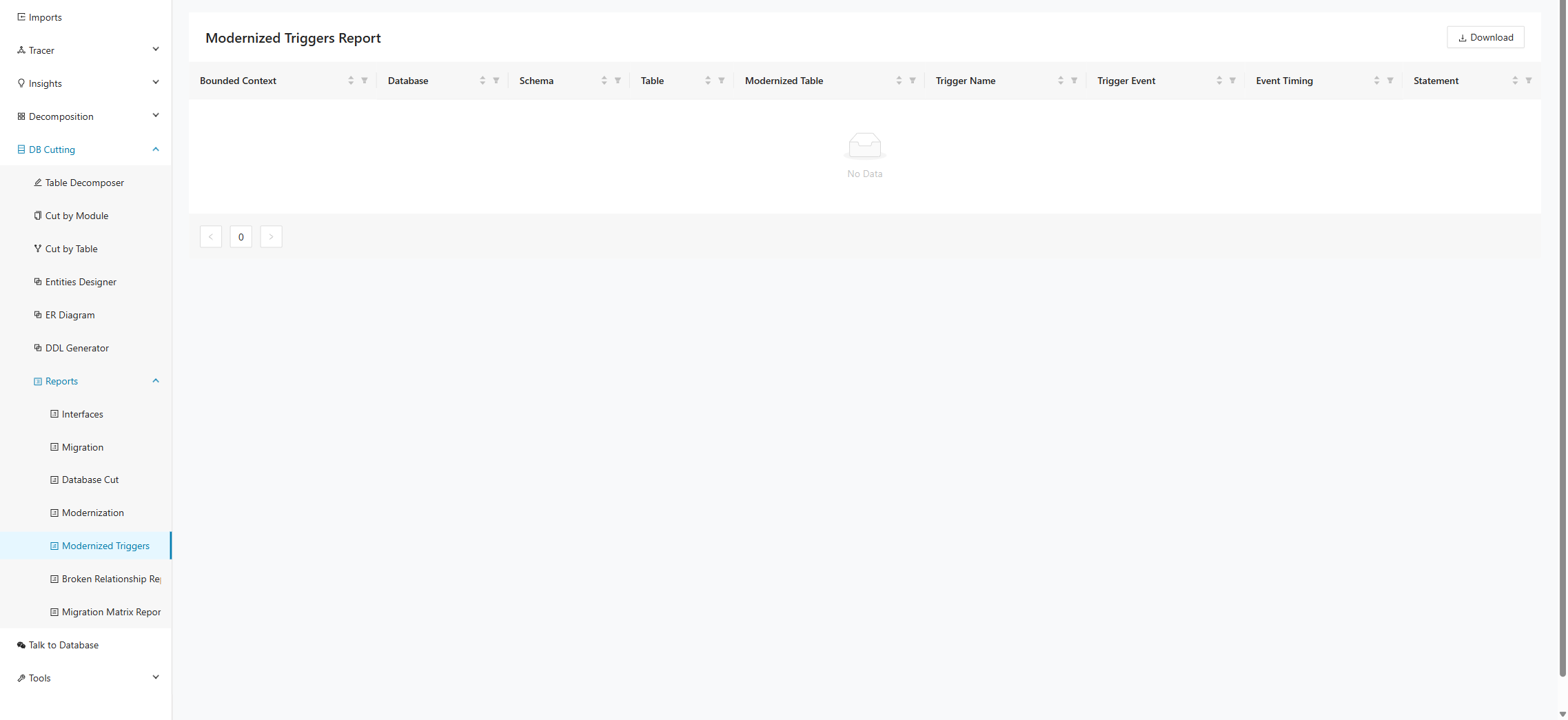
Click Download to export the current table view as a CSV file for use in external tools or further analysis.
Broken Relationship
The Broken Relationship report identifies foreign key relationships between tables that have been broken as a result of the database cut. This occurs when a table with a foreign key reference is assigned to a different bounded context than the table it references, creating a cross-context dependency that no longer holds a direct database relationship. The report helps users identify these inconsistencies so that the appropriate interface or integration strategy can be applied. All columns are sortable and can be filtered.
The table contains the following columns:
- Bounded Context 1 identifies the bounded context that owns the table containing the foreign key.
- Table 1 identifies the table that holds the foreign key reference.
- Foreign Column 1 identifies the foreign key column in Table 1.
- Bounded Context 2 identifies the bounded context that owns the referenced table.
- Table 2 identifies the table being referenced by the foreign key.
- Foreign Column 2 identifies the referenced column in Table 2.

Click Download to export the current table view as a CSV file for use in external tools or further analysis.
Migration Matrix report
The Migration Matrix report provides a side-by-side matrix of database columns and bounded contexts. Use this report to compare how the same source tables and columns are represented across multiple bounded contexts and to quickly spot overlaps or gaps in the database cut.
The table contains the following columns:
- Database identifies the source database.
- Schema identifies the source schema.
- Table identifies the source table.
- Column identifies the source column.
- Bounded Context columns display one column per bounded context so you can compare the same source column across all contexts in a single view.
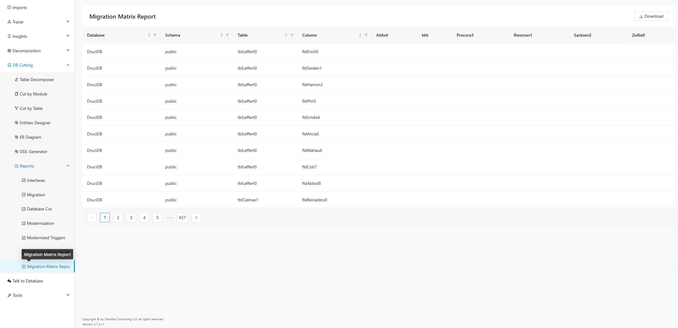
Click Download to export the current matrix for use in analysis, review sessions, or downstream tooling.
Code Generator
After you create clients and projects and import the required files, you can use the Code Generator features described on this page. Decompose uses the imported database and application knowledge to drive AI-supported code generation for modernization tasks. This page explains how each generator area works so you can configure the right inputs and review the generated outputs effectively.
Tech Stack
The page is a questionnaire for gathering information about a database modernization project. It collects details about the legacy and target databases, the tools and frameworks used for migration, and the programming languages involved. The specific information collected includes:
-
Legacy database type
-
Target database type
-
Database migration tool
-
Database migration framework
-
Database migration language
-
Programming language of the modernized application
-
Object-Relational-Mapping framework
-
Web framework
-
Desired cloud provider, region and deployment environment
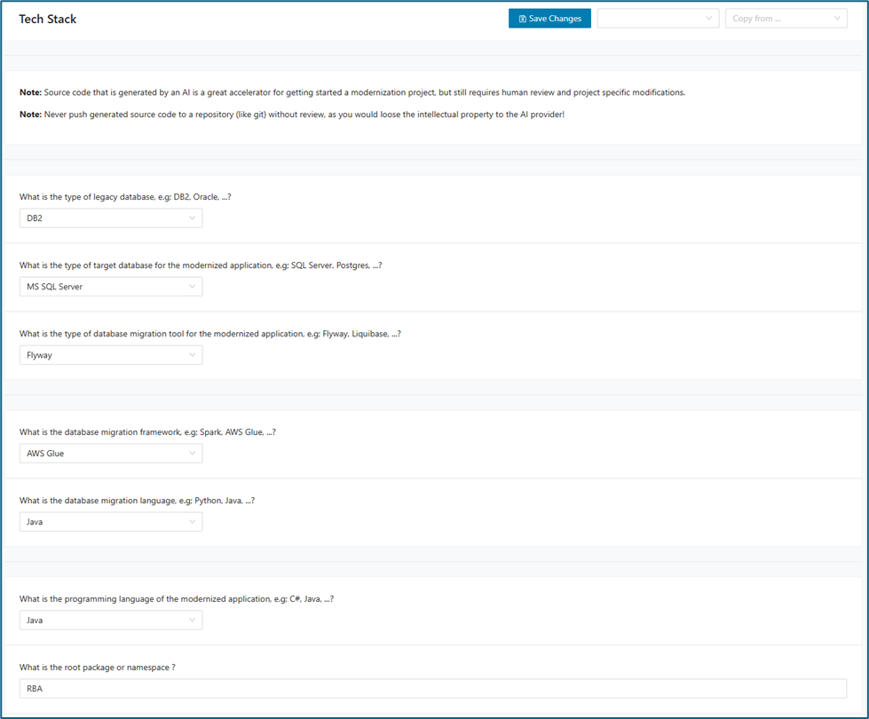
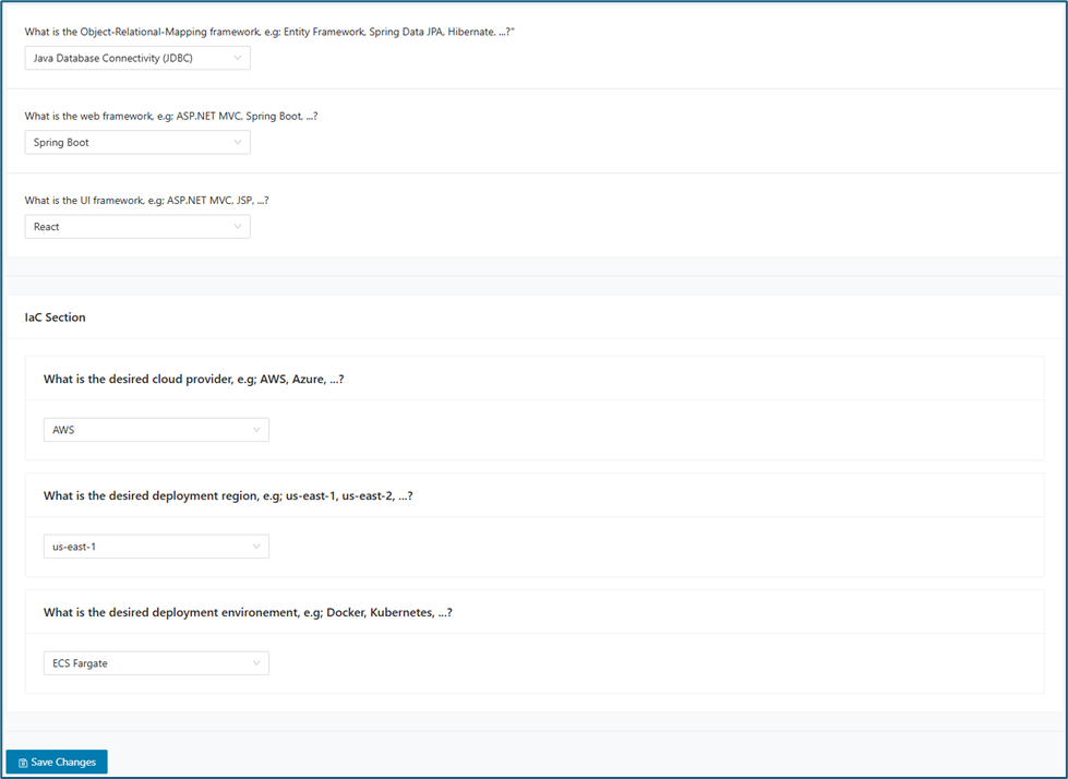
You can save tech stack preferences for a specific bounded context or table.
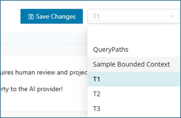
You can copy an existing tech stack from your saved preferences. Select the desired tech stack in the Copy from... drop-down, choose the destination where you want to apply it, and then click Save. The following screenshot highlights the Copy from... drop-down:
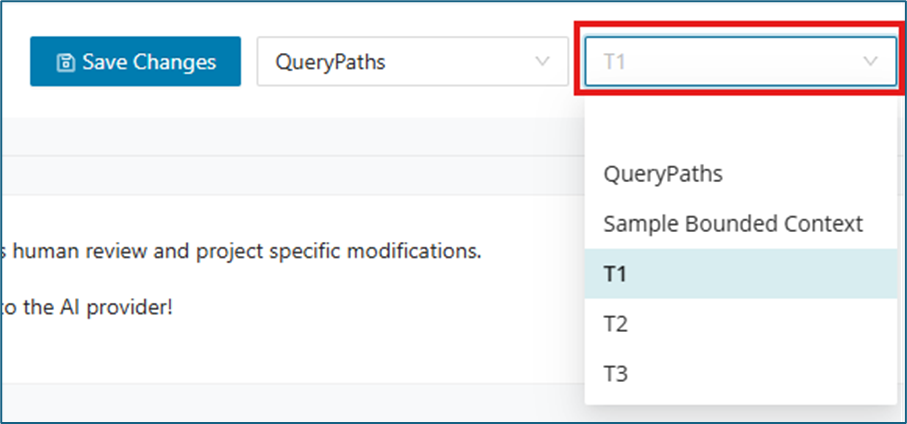
SQL Queries
On the Query Generator page, leverage GenAI to automatically translate SQL queries from your legacy database into equivalent queries for your modernized database. In addition to query conversion, GenAI also generates the source code required to invoke these new queries directly from your modernized application stack.
Queries are organized by business module and table. Each module and table is displayed in its own dedicated tab, making it simple to navigate between sections. Within every tab, you'll find both the original queries and their GenAI-generated modern equivalents, along with the corresponding invocation code for seamless integration.
To use this feature, select a bounded context or table in the drop-down.
Note: A Tech Stack must be set on that specific Bounded Context or Table to use this feature.

After selecting a Bounded Context or Table, all associated Modules and Tables will be loaded automatically in their respective tabs.
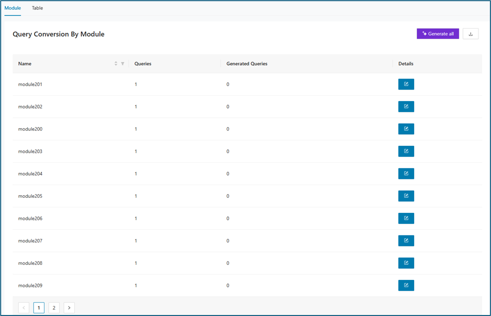
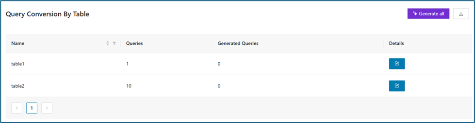
When the button on the Details column is clicked, the generated queries will be displayed.
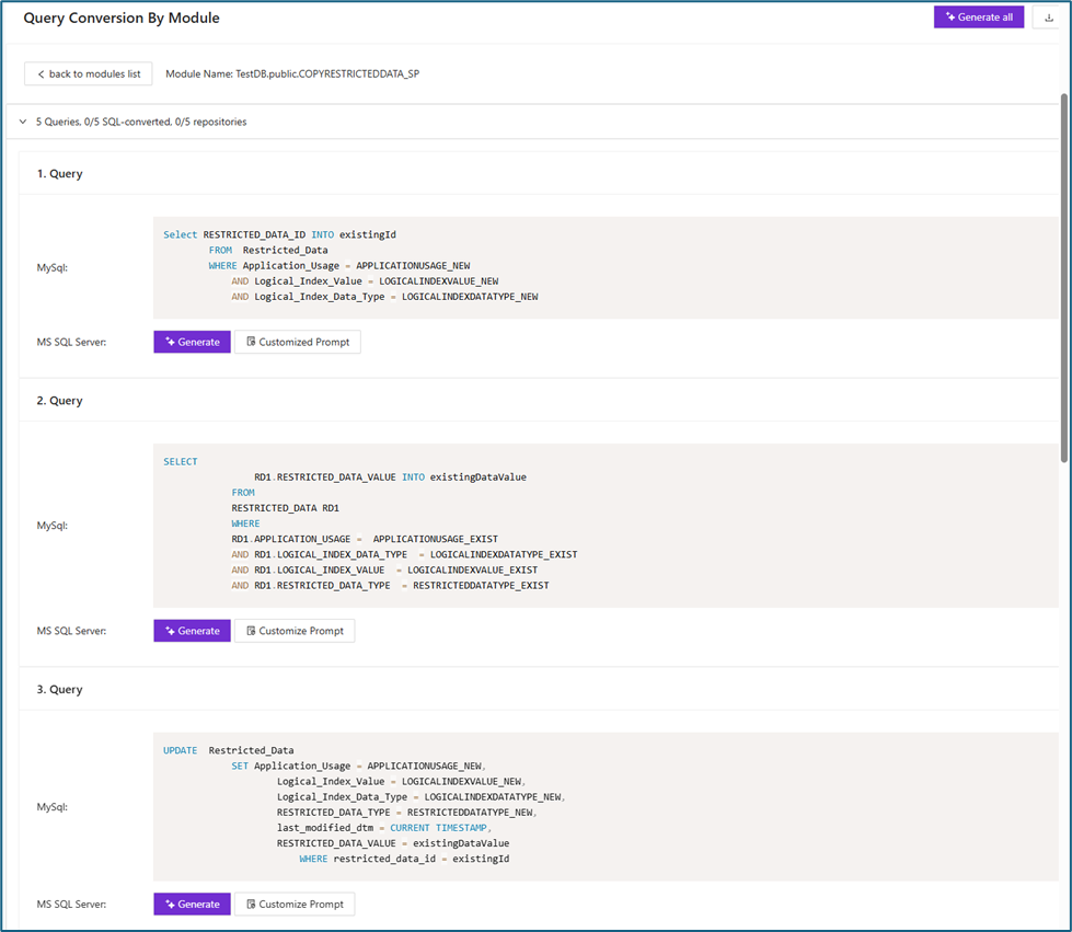
You have multiple options for generating queries. You can click Generate All in the upper right to generate all queries at once, generate each query individually, or customize the prompt for each query as needed.
When you click Customized Prompt, you can give the AI more specific instructions.
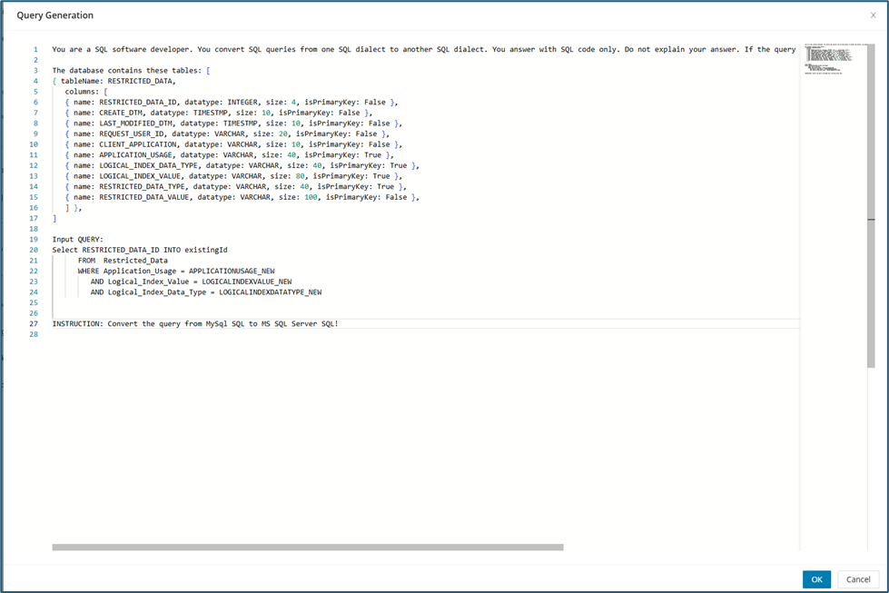
Stored Procedures
The Stored Procedures view is available in the current Code Generator UI. The following screenshot shows the page layout for this area.
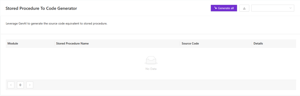
Database Layer
This feature automates the creation of the Database Layer for existing legacy database tables. Instead of manually writing code to connect to each old table, this tool uses Generative AI (GenAI) to produce the required code structures for selected tables.
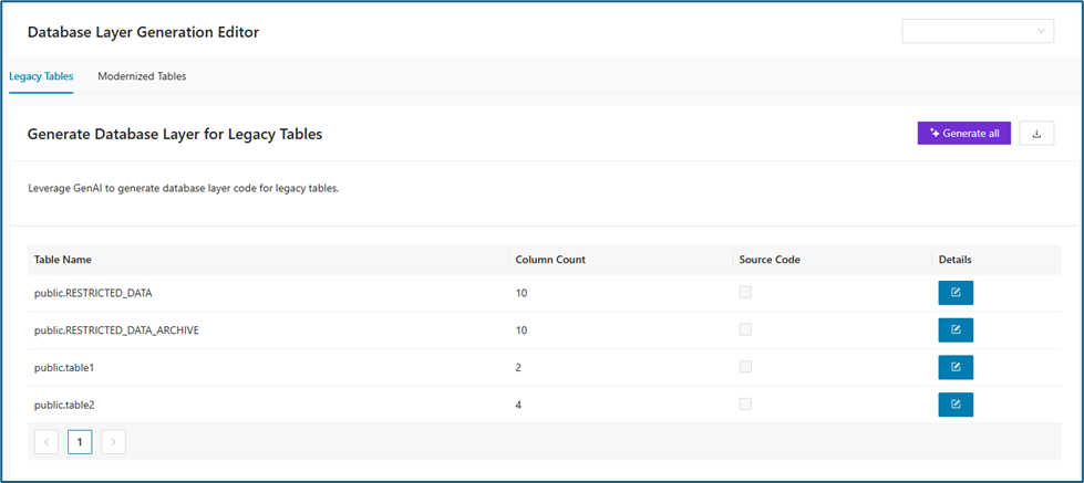
Clicking the edit icon in the Details column displays a breakdown of each table’s columns, including column names, data types, and primary key information. To instantly generate the corresponding database layer code, simply select either the Generate button for an individual table or the Generate All button for bulk creation. The code will be automatically produced in the programming language and framework you selected on the Tech Stack tab.
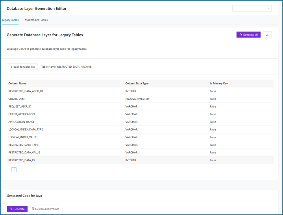
You can also customize the AI code generator instructions by clicking Customized Prompt. This lets you tailor the generated code to specific requirements.
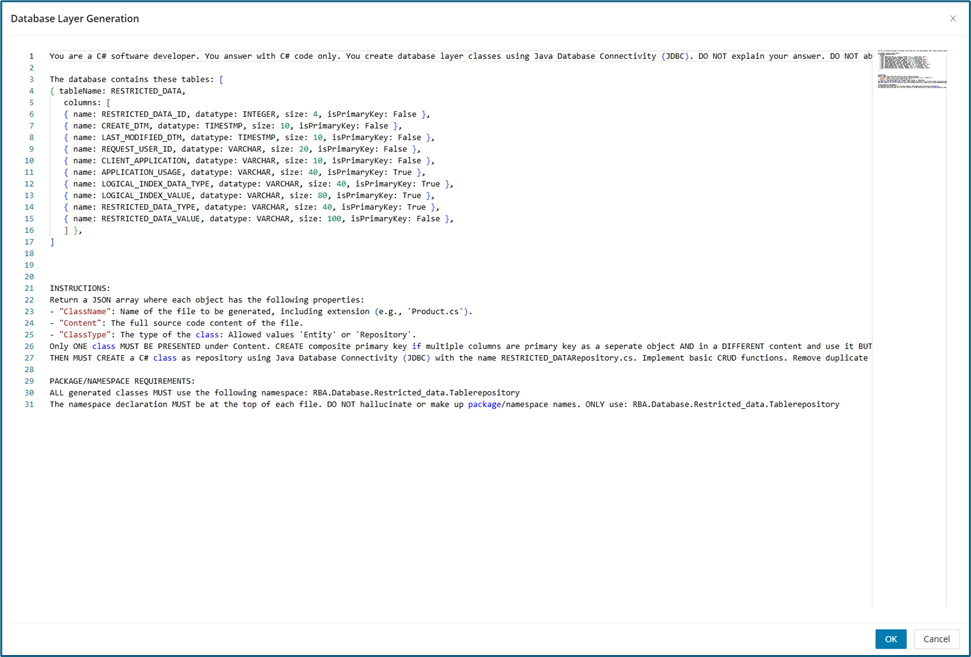
Once code generation is complete, the results appear at the bottom of the page. You can review, copy, or edit the code as needed. In some cases, multiple code blocks are generated so that you can work with different sections individually.
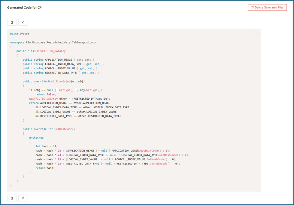
To edit the generated code, simply click the edit icon and make any necessary changes.

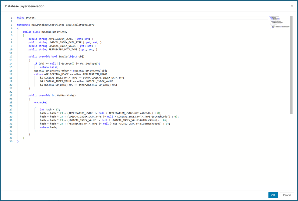
Modernized Tables
The Modernized Tables tab shows tables that have been updated or generated by the tool. Tables appear here after the cutting process is completed through DB Cutting. In this section, you can view the source code for each modernized table together with additional details about its structure and configuration. Select the required Bounded Context or Table from the upper-right drop-down.
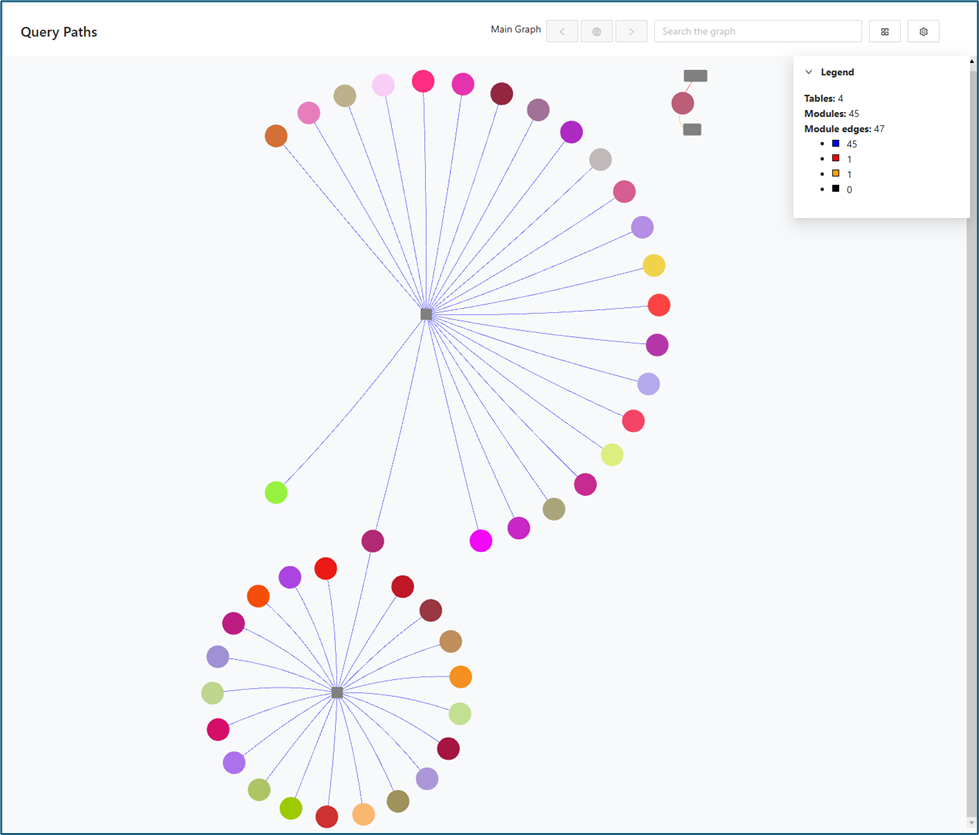
When the Generate All is clicked, the tool will generate the relevant code for all tables. The generated code for each table can then be viewed by clicking Details .
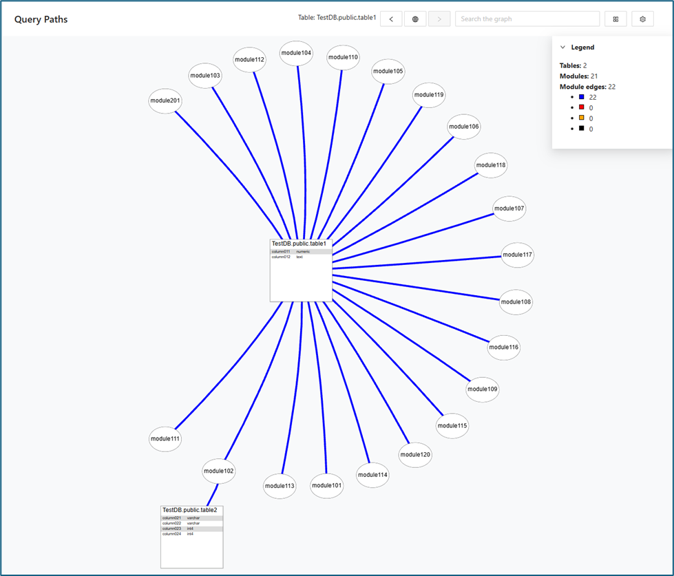
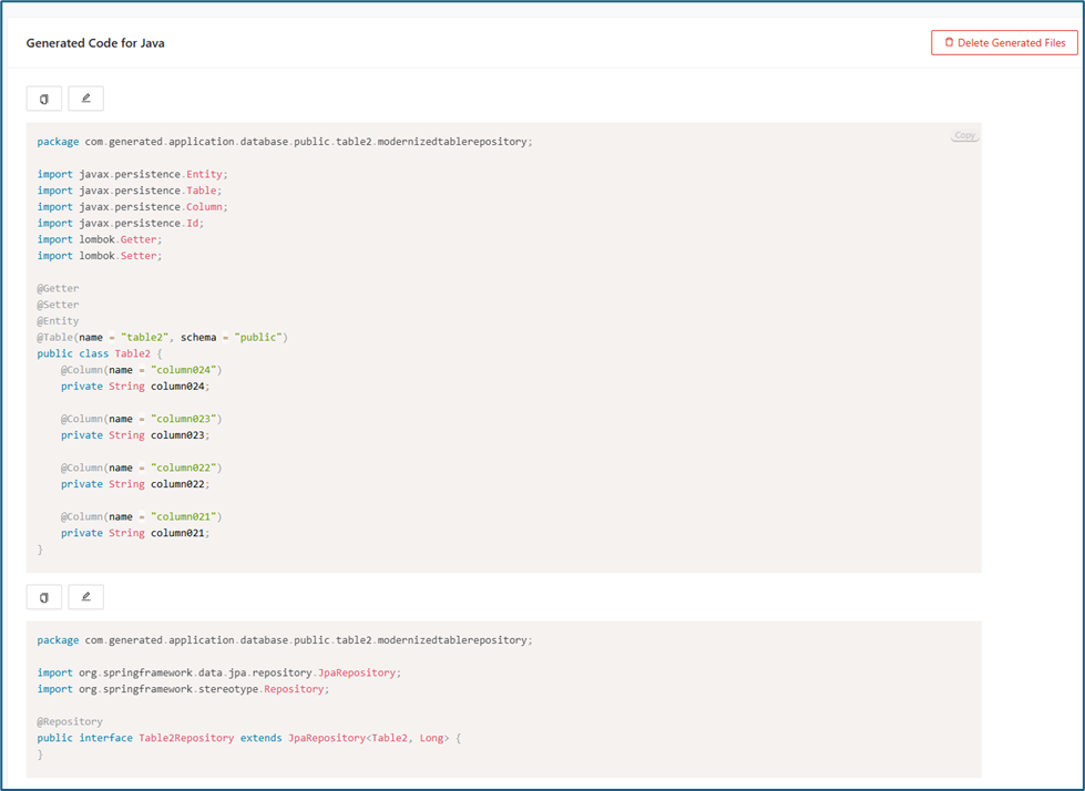
Service Layer
The Service Layer Generation is designed to further streamline and automate modernization projects by generating the “service layer” code that sits on top of the database layer for legacy tables. This feature leverages GenAI to create standardized, efficient service logic for interacting with legacy databases—a critical step in rebuilding or replatforming older systems.
To use the Service Layer feature, first generate the code for the Database Layer. This ensures that all necessary database components are in place.
In the Legacy Tables section, you’ll find the generated code for the database layer. In this example, code for the RESTRICTED_DATA table has already been generated and is displayed here. As you generate code for additional tables, each one will appear as its own row in the Legacy Tables list.
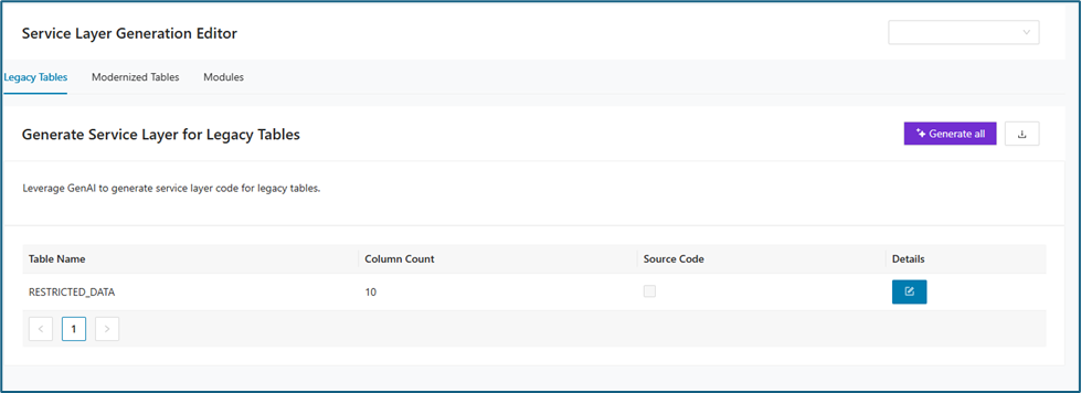
To view or copy the generated code, click the edit icon in the Details column. The first panel displays the Generated Repository Codes.
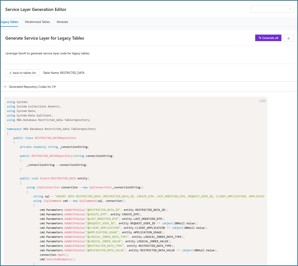
When you click either the Generate All or Generate button, the code generation process for the service layer will begin. Once complete, the second panel will display the generated service codes.
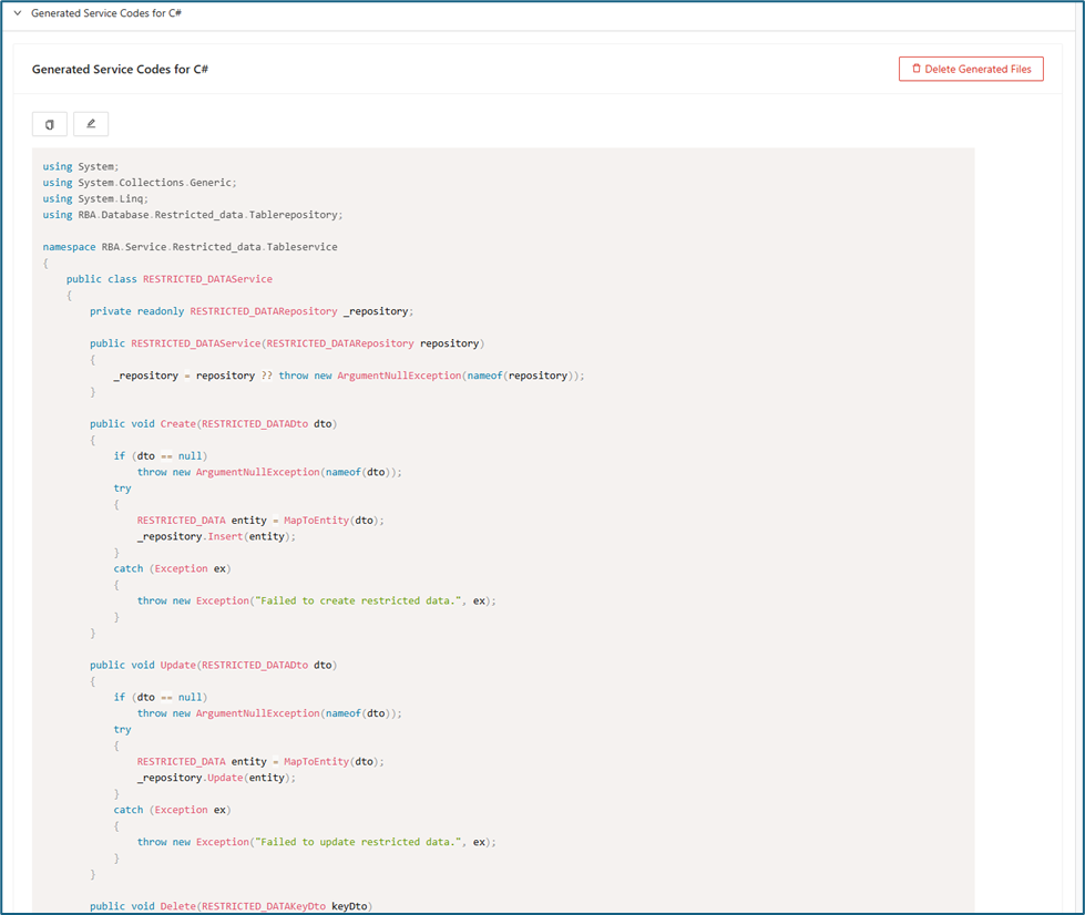
Modernized Tables
The Modernized Tables tab shows tables that have been updated or generated by the tool. Tables appear here after the cutting process is completed through DB Cutting. In this section, you can view the source code for each modernized table together with additional details about its structure and configuration. Select the required Bounded Context or Table from the upper-right drop-down.
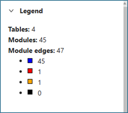
When the Details button is clicked on a specific row, the generated repository code for that table will be displayed. Clicking Generate All will generate the corresponding service code for the selected table.
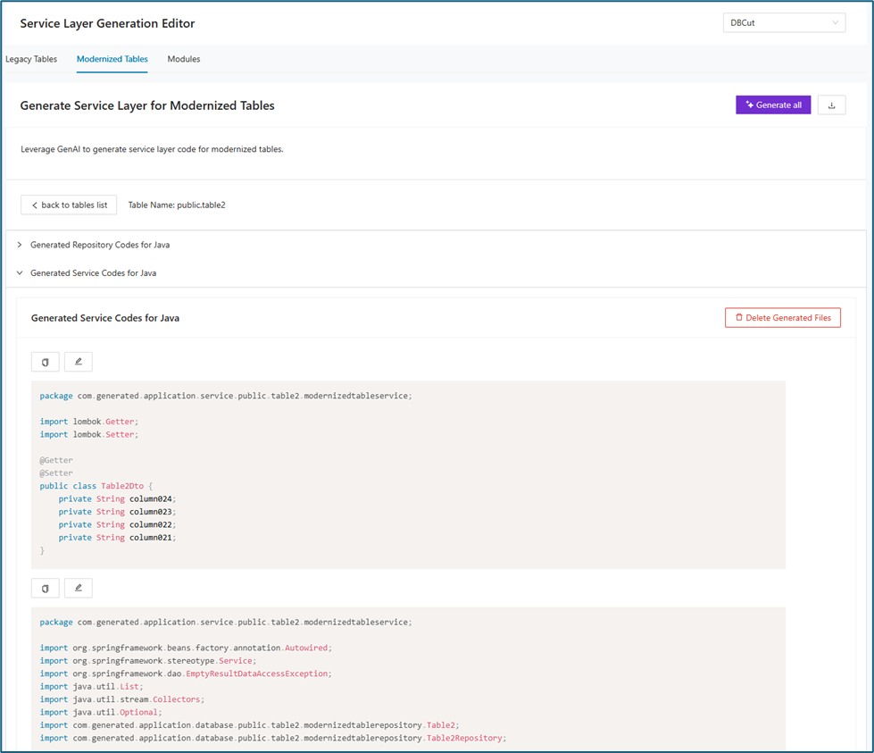
Modules
The Modules tab shows modules that have been updated or generated by the tool. Select the required Bounded Context or Table from the upper-right drop-down.
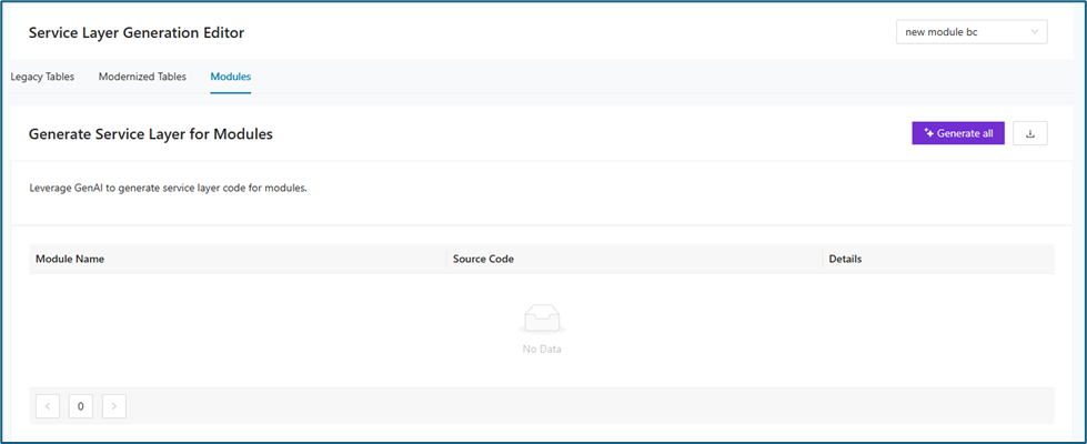
API Layer
The API Layer Generation Editor is designed to automate the creation of the API endpoints that expose legacy table data and business functionality to external systems, applications, or user interfaces. Using Generative AI (GenAI), this feature builds a fully functional API layer, facilitating a smooth modernization of legacy systems and aligning them with today’s best practices for connectivity, security, and scalability.
To use the API Layer feature, first generate the code for the Service Layer. This ensures that the required supporting components are already in place.
In the Legacy Tables section, you’ll find the generated code for the service layer. In this example, code for the RESTRICTED_DATA table has already been generated and is displayed here. As you generate code for additional tables, each one will appear as its own row in the Legacy Tables list.
To view or copy the generated code, click the edit icon in the Details column. The first panel displays the Generated Service Codes.
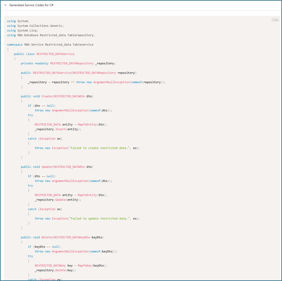
When you click either the Generate All or Generate button, the code generation process for the service layer will begin.
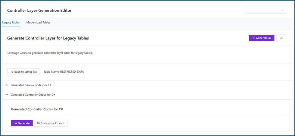
Once complete, the second panel displays the generated API code.
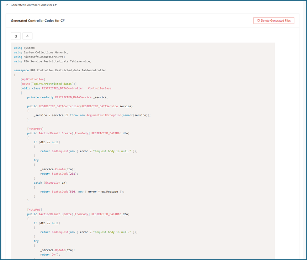
Modernized Tables
The Modernized Tables tab shows tables that have been updated or generated by the tool. Tables appear here after the cutting process is completed through DB Cutting. In this section, you can view the source code for each modernized table together with additional details about its structure and configuration. Select the required Bounded Context or Table from the upper-right drop-down.
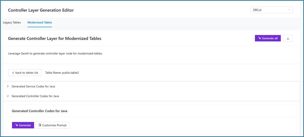
When Details is clicked on a specific row, the generated service code/s for that table will be displayed. Clicking Generate All button will generate the corresponding controller code for the selected table.
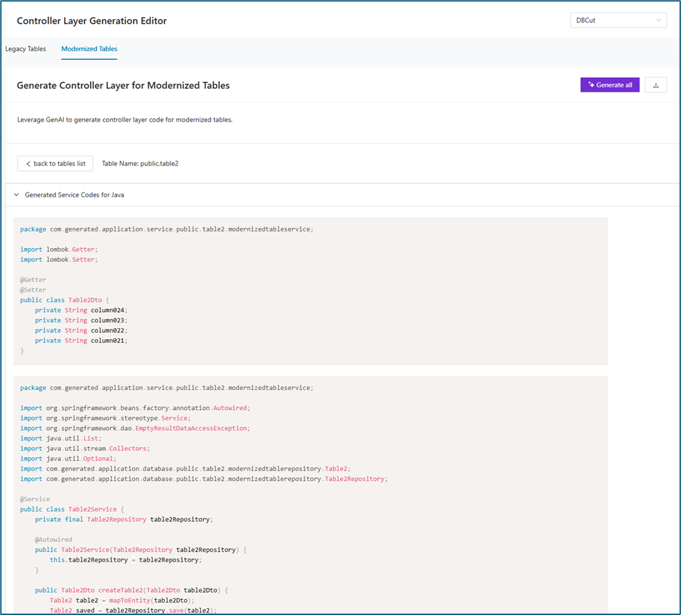
Here's the generated controller code:
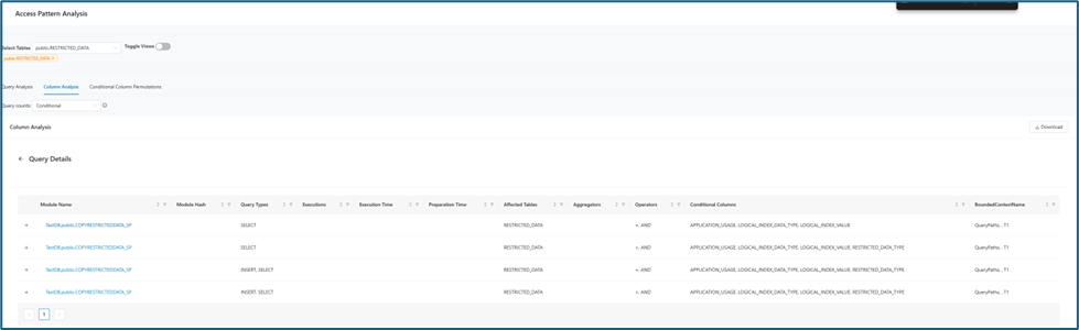
Dependency Tree
This feature leverages Generative AI to modernize legacy code by generating updated source code along with all required dependencies. The table below displays all modules included within the selected bounded context.
Note: Before using this feature, please complete the following steps:
-
Import the Module Source Code and Module Relations CSV files to establish the dependency tree among modules.
-
Create a Bounded Context that includes all related modules.
-
Set your preferred technology stack within the created Bounded Context.
-
Click on Dependency Tree tab then Select the Bounded Context from the dropdown menu. This will display a table similar to the one shown below.
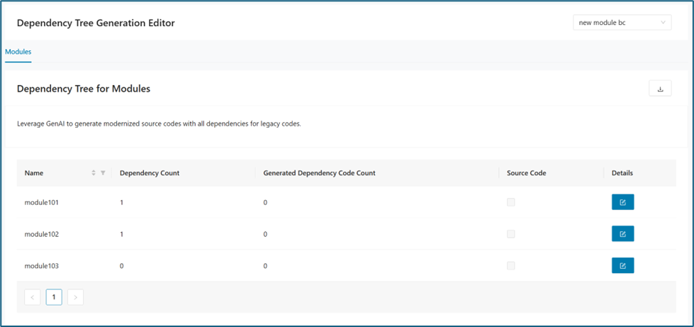
When the button in the Details column is clicked, any associated dependencies (if the module has dependencies) and the legacy source code will be displayed. To generate modernized code based on your selected language from Technology Stack, simply click Generate .
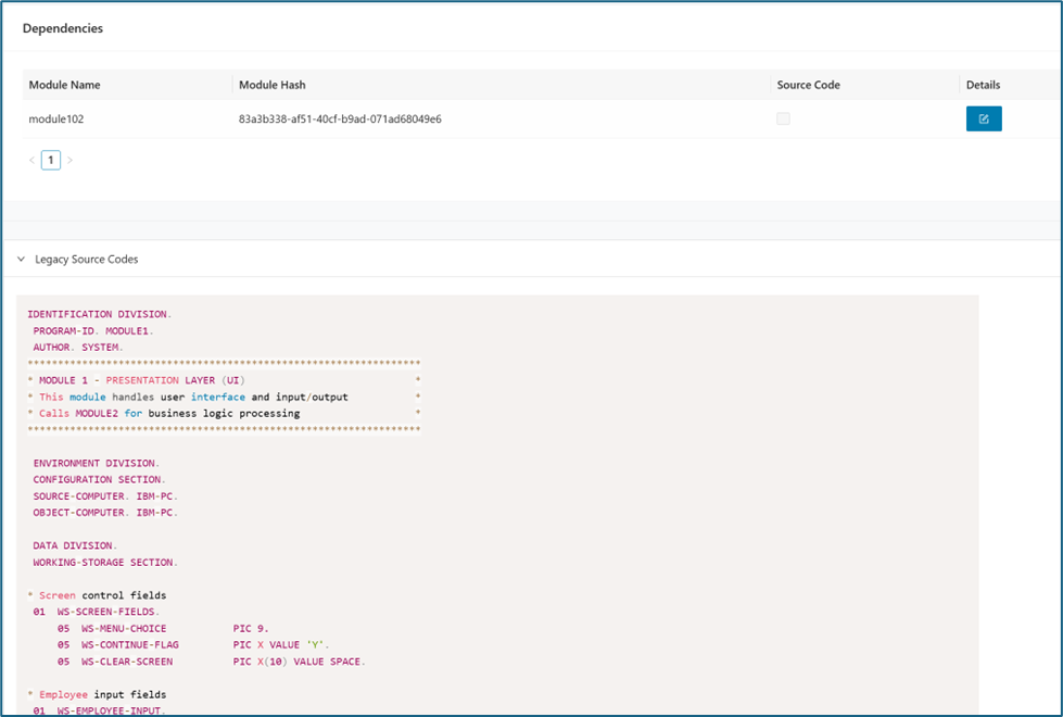
When the code is successfully generated, it is displayed in the bottom panel of the page.
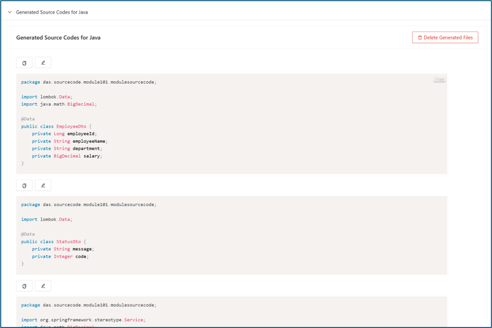
Infrastructure as Code Generator
The Infrastructure as Code Generator is an experimental feature of the Decompose platform that automates and streamlines the creation, validation, and visualization of production-grade Infrastructure as Code (IaC) on Terraform. This tool harnesses structured metadata produced by Decompose’s bounded context extraction, leveraging large language models (LLMs) for code generation, iterative error correction, and automated architecture diagram synthesis. By integrating these advanced capabilities, the tool accelerates IaC delivery while supporting high-quality, maintainable infrastructure designs. Here are Infrastructure as Code Generator's key features:
-
Automated IaC Generation
- Terraform Decompose takes structured metadata related to microservices—such as service relationships, database requirements, and infrastructure dependencies—and translates it into validated Terraform code following best practices. The result is a ready-to-deploy, production-grade IaC setup.
-
Iterative Error Correction
- The system automatically detects syntax or configuration errors using terraform validate. Upon failure, it extracts diagnostic output and invokes the LLM to iteratively fix the issues. This process is repeated automatically (up to 10 times by default), ensuring correctness with minimal human involvement.
-
Architecture Diagram Generation
- Terraform Decompose uses the terraform graph -type=plan command to generate DOT-formatted infrastructure graphs. These are then converted into Mermaid.js syntax, producing clean and easy-to-understand architectural diagrams suitable for documentation or visualization purposes.
-
Agentic Workflow
- The workflow is managed by an autonomous agent that decomposes the task into subtasks, handles retries, interprets validation errors, and integrates feedback without manual intervention.
Info
For the rows to display in Infrastructure as Code tab, all tables and bounded context must have a Tech Stack preference saved.
The Infrastructure as Code (IaC) workflow consists of the following steps:
1. Input: Bounded Context Metadata
Receives structured metadata for all bounded contexts (microservices) from Decompose, including:
-
Service names
-
Service relationships and dependencies
-
Estimated table counts
-
Deployment/environment details
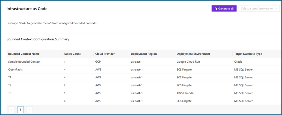
2. Initial IaC Generation
Based on the metadata and user-defined parameters (cloud provider, resource types, networking settings, etc.), the LLM generates all foundational Terraform files:
-
provider.tf
-
variables.tf
-
terraform.tfvars
-
main.tf
-
output.tf
Choose on a terraform version and click Generate All , the IaC Generation Progress Bar will then appear.
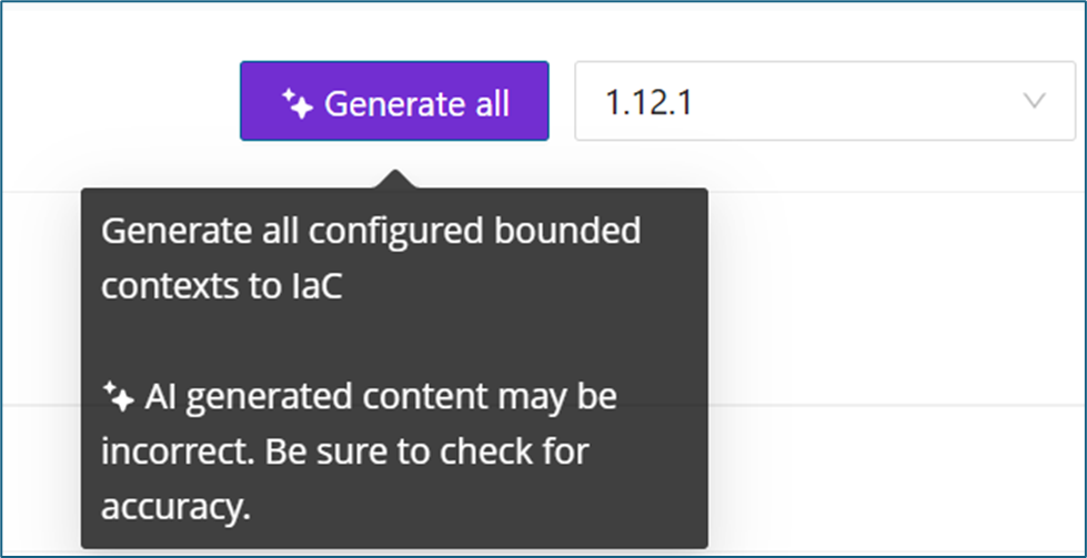

3. Validation Loop
-
Executes terraform init and terraform validate on the generated files.
-
On validation failure, error diagnostics are captured and sent back to the LLM.
-
The files are regenerated based on the feedback, repeating the process for up to 10 iterations.

If validation fails, a Fix with AI button will appear, enabling you to automatically address the detected errors. When clicked, the system will initiate the correction loop again, allowing iterative fixes until validation succeeds.
4. Diagram and Code Generation
-
Once validation succeeds, the tool runs terraform graph -type=plan to produce the infrastructure graph in DOT format.
-
This output is parsed and converted to Mermaid.js diagrams, providing a human-readable architecture overview.
Migration Generator
The Migration Generator helps you create and review migration assets for a selected bounded context. In one place, you can generate database creation scripts, data migration scripts, and query equality test artifacts for legacy and modernized data models.
Note
Use this page after you select your working project and bounded context. The bounded context must also have a saved Tech Stack.
DB Creation Scripts
Use DB Creation Scripts to generate DDL assets for both legacy and modernized tables in the selected bounded context. This tab helps you create the structural database artifacts needed for implementation and review. Use it when you want to inspect, generate, or validate table and relation scripts before downstream migration work. This tab provides:
- A Legacy Tables sub-tab and a Modernized Tables sub-tab
- Bulk actions for Generate all tables and Generate all relations
- Row-level status for generated table scripts and relation scripts
- A Details action for table-level inspection and generation
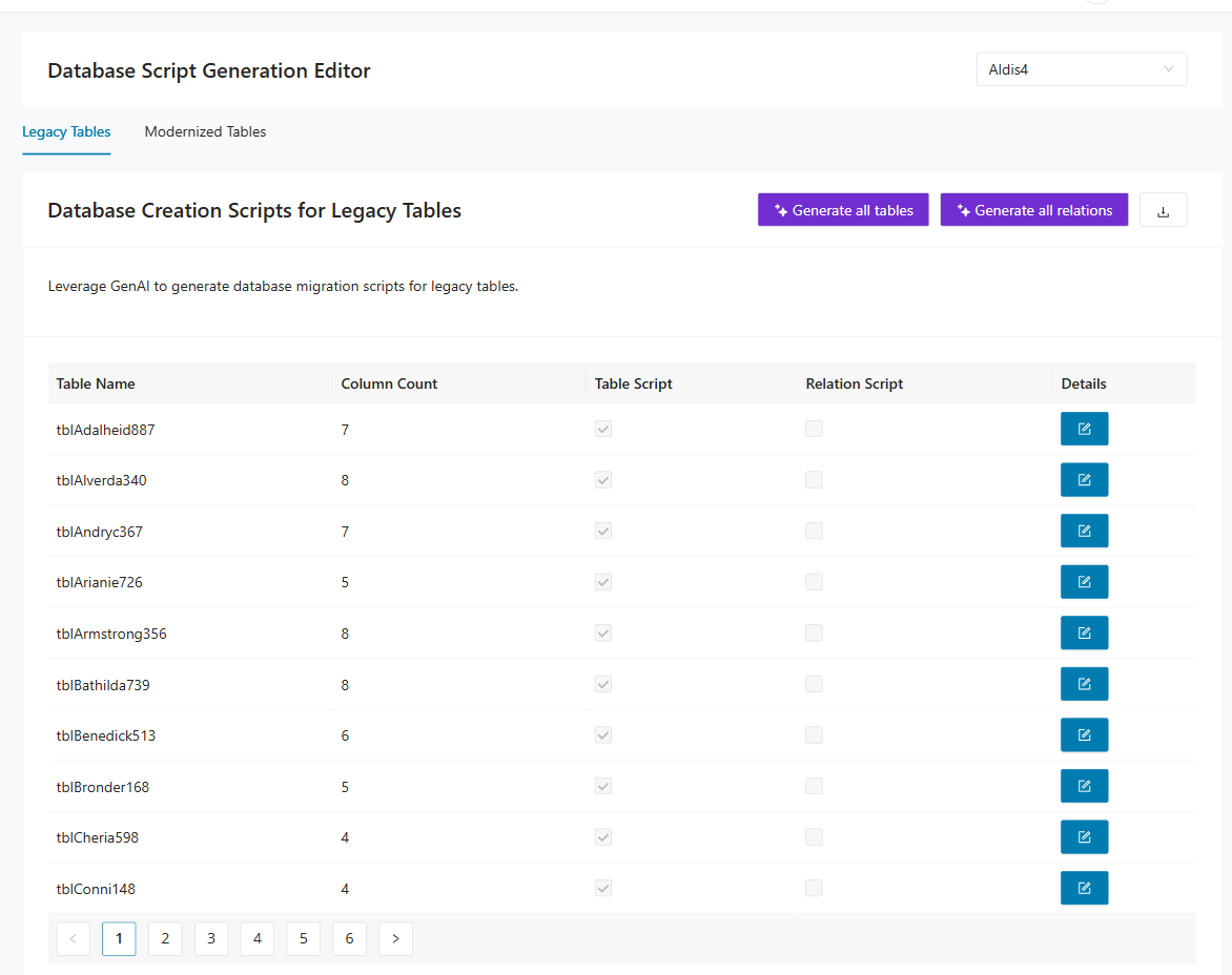
How to use DB Creation Scripts
Select the bounded context from the selector in the upper-right area in Migration Generator > DB Creation Scripts, then choose either Legacy Tables or Modernized Tables. Select Generate all tables to create table DDL in bulk and Generate all relations to create relationship scripts in bulk.
Explore details in Legacy Tables
When you select Details on a legacy table row, the page shows a table-level work area with:
- The selected Table Name and a back to tables list action
- A column metadata grid (Column Name, Column Data Type, Is Primary Key)
- A Generated table script panel
- A Generated relation script panel
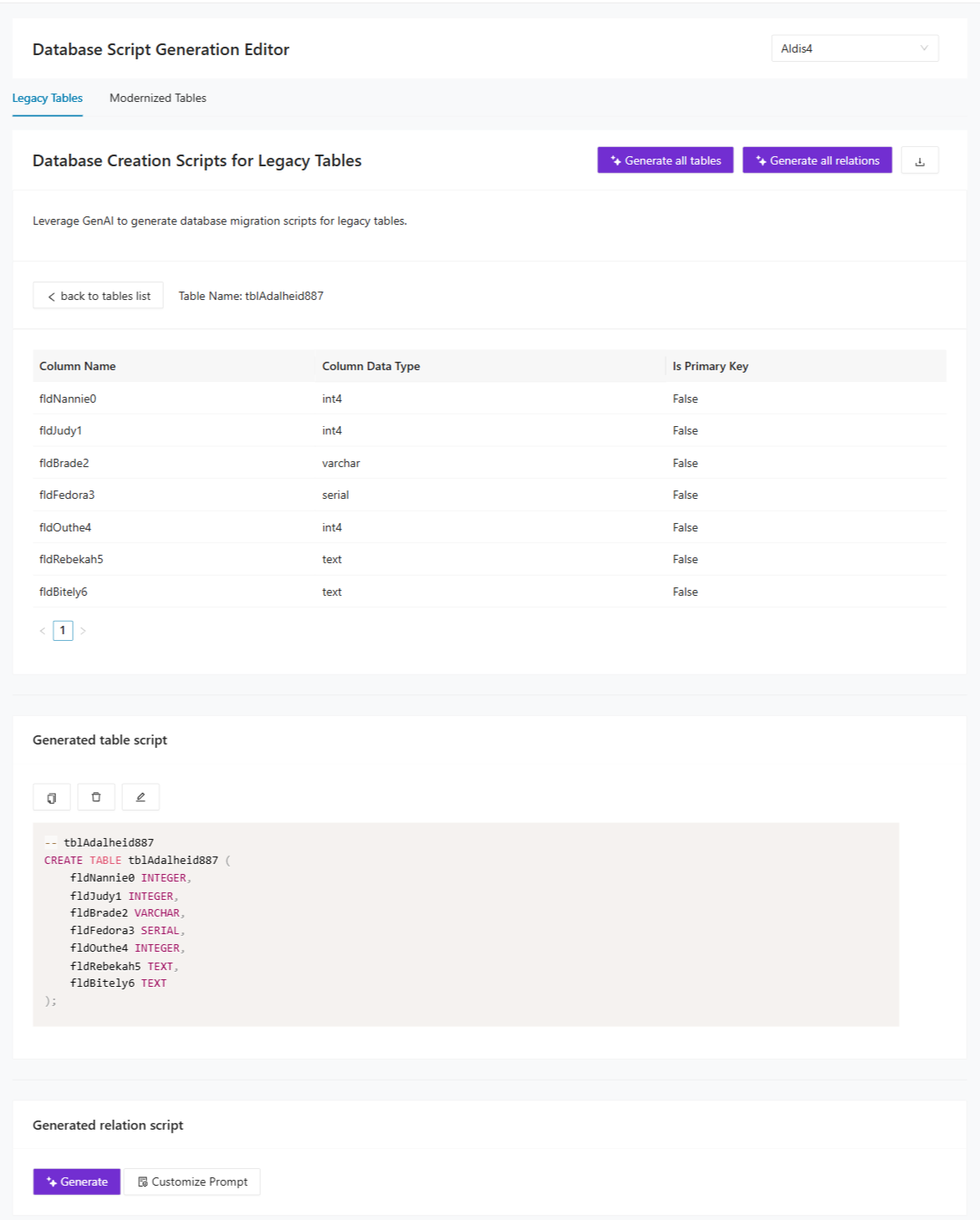
Explore details in Modernized Tables
When you switch to Modernized Tables and open Details for a row, you can inspect the modernized table structure and generate script outputs for that specific table.
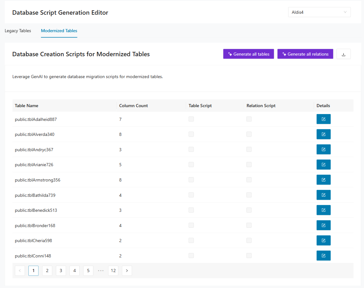
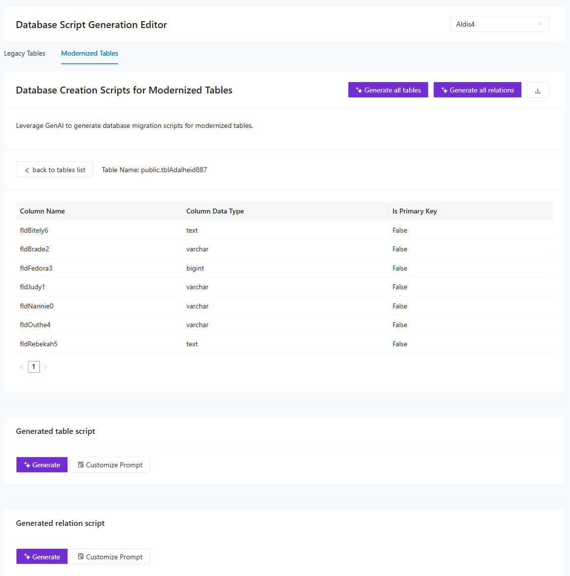
Expected result: You can verify table-level structure, generate DDL artifacts in bulk or per table, and validate script coverage for both legacy and modernized scopes.
Data Migration Scripts
Use Data Migration Scripts to generate executable migration logic that moves data from legacy tables to modernized targets. It focuses on the transformation logic required to populate the new data model from the legacy source. Use it when you are ready to inspect or generate the code that performs table-level migration. This tab provides:
- A Generate all action for bulk migration script generation
- A table-level status grid with row-level diagnostics
- A Details drawer for each row with metadata and generated script content
- A Selection action for targeted table operations
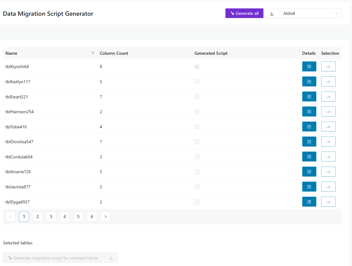
How to use Data Migration Scripts
Select the bounded context in Migration Generator > Data Migration Scripts, then select Generate all to run migration script generation for all listed rows. To inspect metadata and generated code for a specific table, select Details for that row.
Explore details in Data Migration Scripts
The Details drawer provides:
- The selected table name
- Source column metadata (Column Name, Column Data Type, Is Primary Key)
- A Generated Data Migration Script panel that shows generated code
- Row-level generation actions, including Generate migration script for this table and Customize Prompt
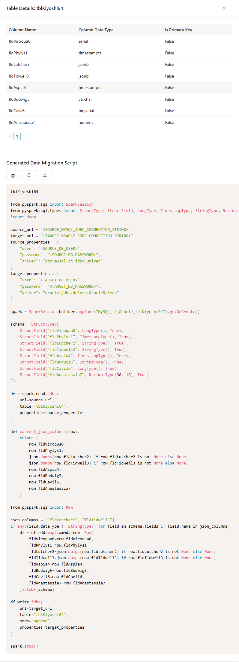
Expected result: You can inspect generated migration logic for each table, verify script completeness, and regenerate or customize prompts where needed.
Query Equality Tests
Use Query Equality Tests to compare legacy query behavior with modernized query behavior and to generate related test artifacts. This area helps you verify that generated modernization outputs still behave correctly against the intended query semantics. Use it when you need evidence that query conversion and generated tests are ready for review. This tab provides:
- A Generate all action for query conversion and test-generation tasks.
- Module-level progress indicators for generated SQL and unit-test artifacts.
- Row-level Details expansion for query-by-query review.
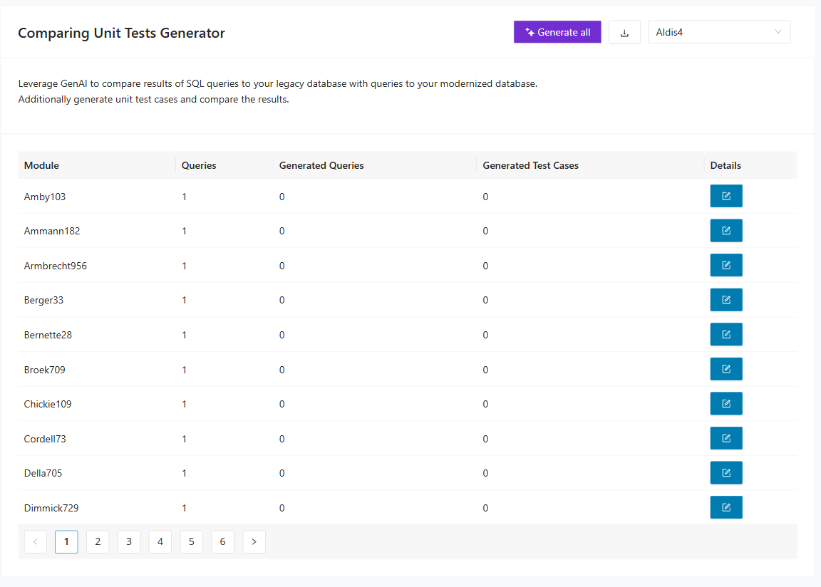
How to use Query Equality Tests
Select the bounded context in Migration Generator > Query Equality Tests, then select Generate all. Open Details for a module to inspect query-specific outputs and confirm query conversion and test-generation progress.
Explore details in Query Equality Tests
The module details area shows:
- Query counts and generation status per module
- The source query (for example, MySQL)
- Target query generation action (for example, Oracle > Generate)
- A language-specific output area (for example, Java) for generated test scaffolding
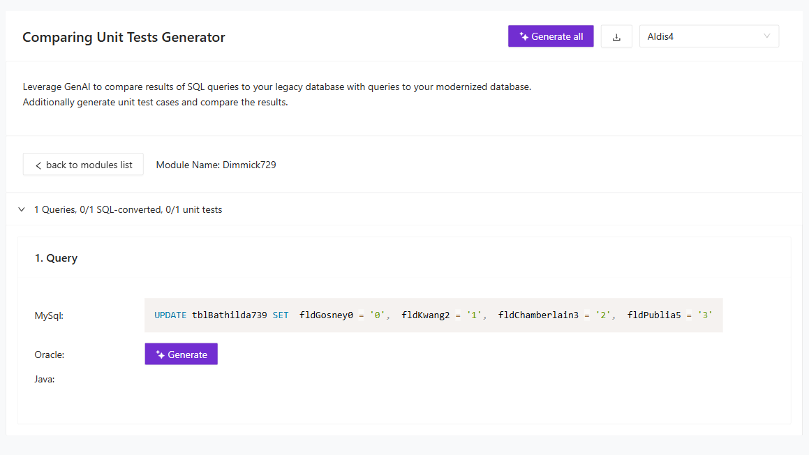
Expected result: You have module-level evidence of query conversion status and test-generation readiness for equality validation.
Downloading scripts
This section explains how to collect the generated outputs after script creation completes. It covers both bulk downloads and targeted downloads for selected migration rows. Use it when you want to package the generated assets for review, handoff, or execution outside the UI.
Select Generate all tables to generate scripts for all tables in the table list. If processing takes time, a loading screen appears:
You can also generate table and relation scripts individually. Select Details for a row, then select Generate in Generated table script or Generated relation script. To download every generated file at once, select the download button to save a ZIP archive that contains the corresponding .sql files.
Generate and download selected data migration scripts
Use the Selection column in Data Migration Scripts to choose one or more tables for targeted generation and download. Select the arrow button for each table that you want to include. The selected tables appear in the Selected tables area at the bottom of the page, where you can clear the list, generate scripts for the selected tables, or download the generated scripts.
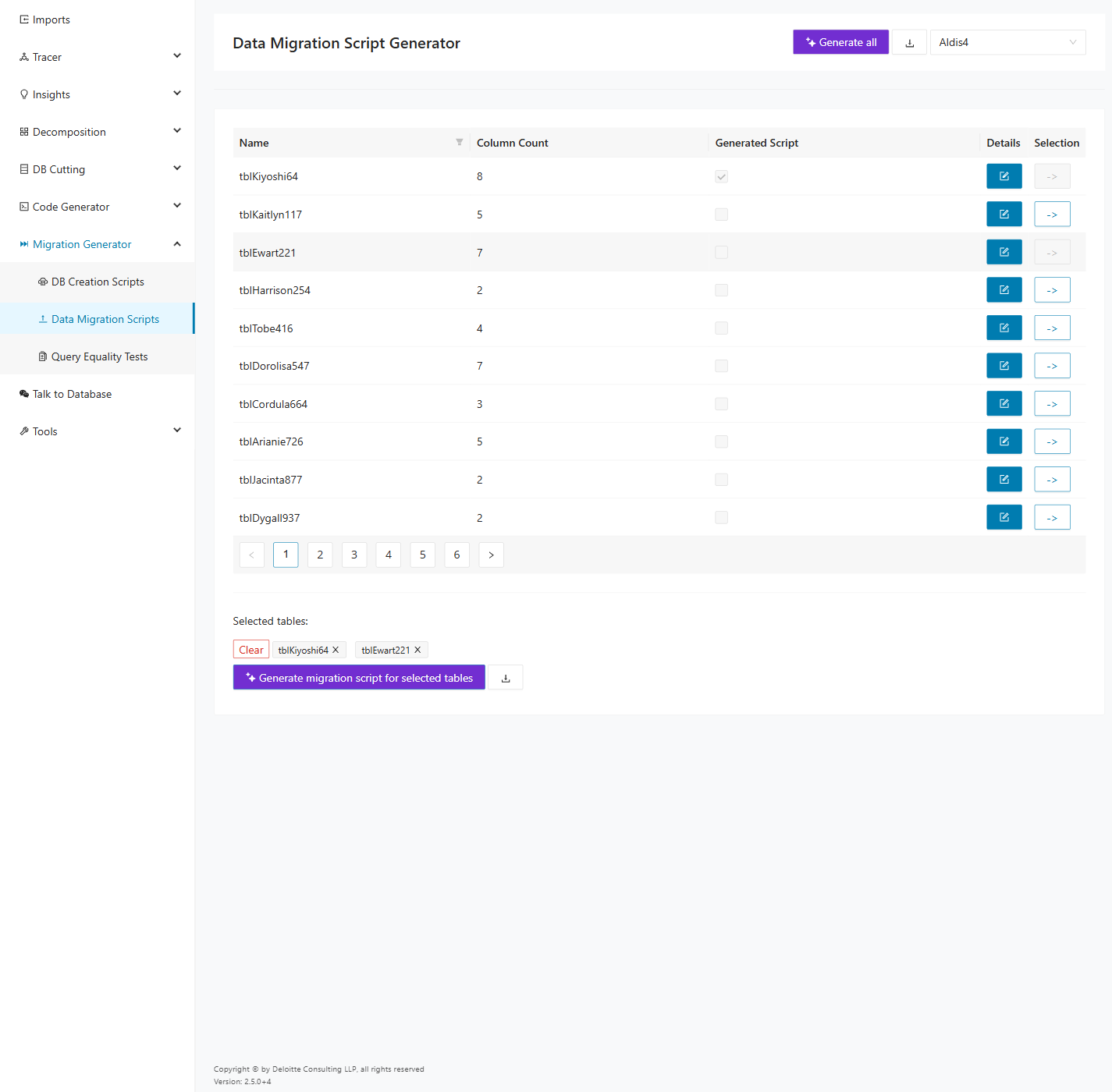
After you select the tables, choose Generate migration script for selected tables to create scripts only for those rows. When generation completes, the Generated Script status is updated for the selected tables and a success message appears.
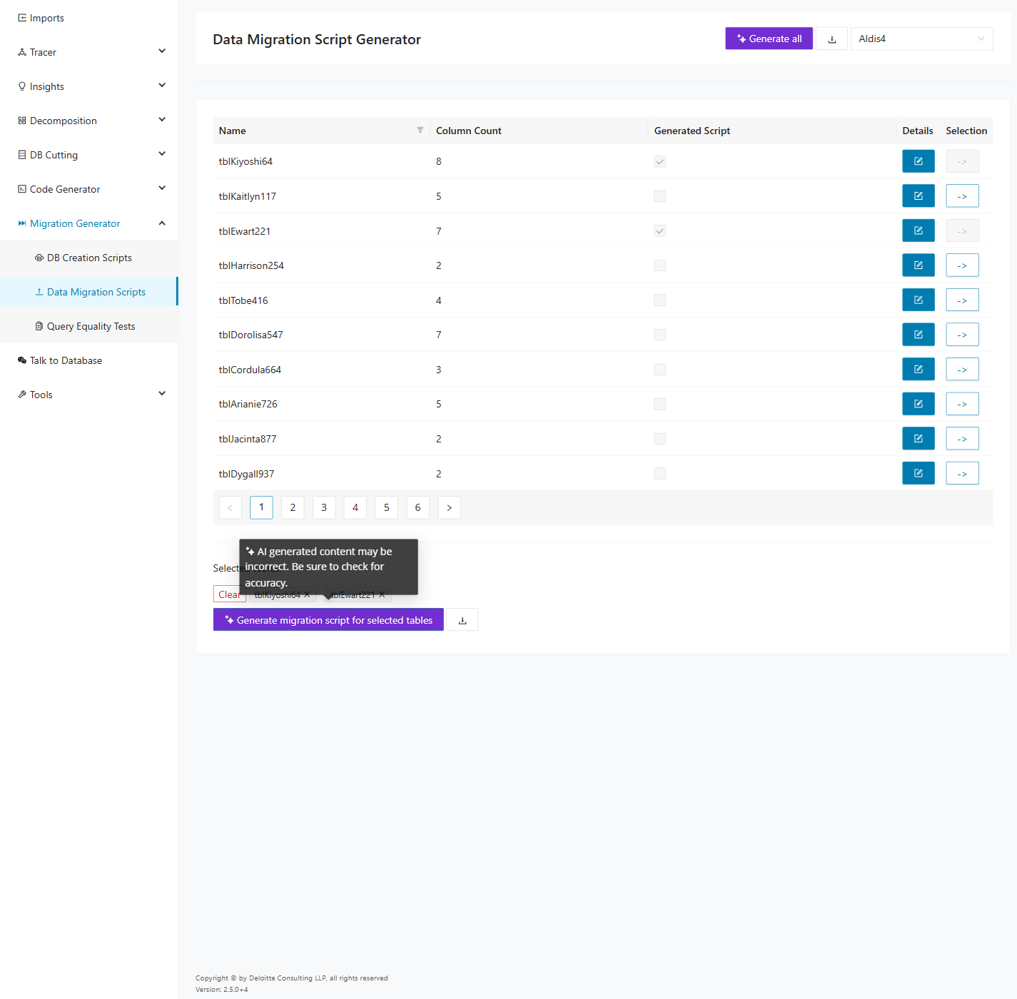
To download the generated scripts for the selected tables, select the download button next to Generate migration script for selected tables. The application downloads a ZIP archive that contains the generated migration scripts for the selected tables.
Tools
The Tools menu provides supporting utilities for maintaining and correcting project data in Decompose. These pages help you validate imported queries, repair schema artifacts, and manage other project-level configuration details. Use them when your workflow requires inspection or cleanup rather than primary decomposition analysis.
SQL Validator
The SQL Validator validates SQL queries for a selected bounded context against modernized databases to display missing columns. It also displays the columns that are part of another context.
To access the SQL Validator, select Tools > SQL Validator in the left navigation panel. Import the schema, bounded contexts, modules, and queries for your project before using this tool.
Selecting a bounded context
Select the desired bounded context from the drop-down list in the upper right corner. After you select a context, the validator populates the query table with all modules assigned to that bounded context. You can switch the bounded context at any time using this drop-down.
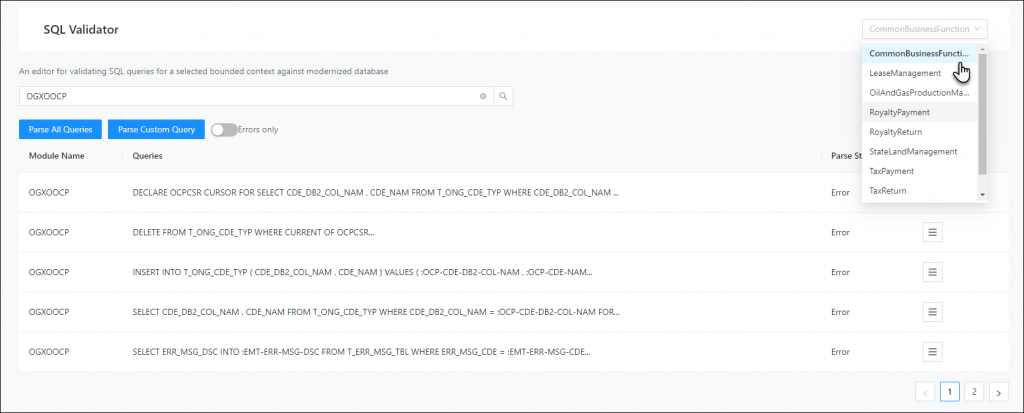
Query table
The main view displays a table of all modules and their queries for the selected bounded context.
| Column | Description |
|---|---|
| Module Names | The name of the module associated with the query. Click the module name to highlight the row. |
| Queries | The SQL query text, truncated if the query is long. |
| Parse Status | The parse result for the query (for example, Success). |
| Missing Columns | The number of columns referenced in the query that are missing from the modernized database. |
| Parse Details | Click the icon to open the parse details view for that query. |
Validating all queries
Click Validate All Queries to parse and validate all queries in the table and update the parse status for each row.
Viewing parse details
Click the icon in the Parse Details column for a query to open the parse details view. This view displays the parsed query with syntax highlighting and line numbers, along with the validation result (for example, Successfully parsed the query against Modernised Database). If the query has missing columns or columns belonging to different contexts, this information is displayed below the query.
Parsing a custom query
Click Parse And Validate Custom Query to open the custom query editor. Enter any SQL query in the code editor and click Parse and Validate Query to validate it against the modernized database. The editor displays the validation result below the query.
Query Editor
The Query Editor is a tool for viewing, modifying, and validating ingested queries. It displays all queries associated with each module and their originating database. Use the Query Editor as a repair tool to update or fix queries that are incorrect or slightly outdated.
To access the Query Editor, select Tools > Query Editor in the left navigation panel.
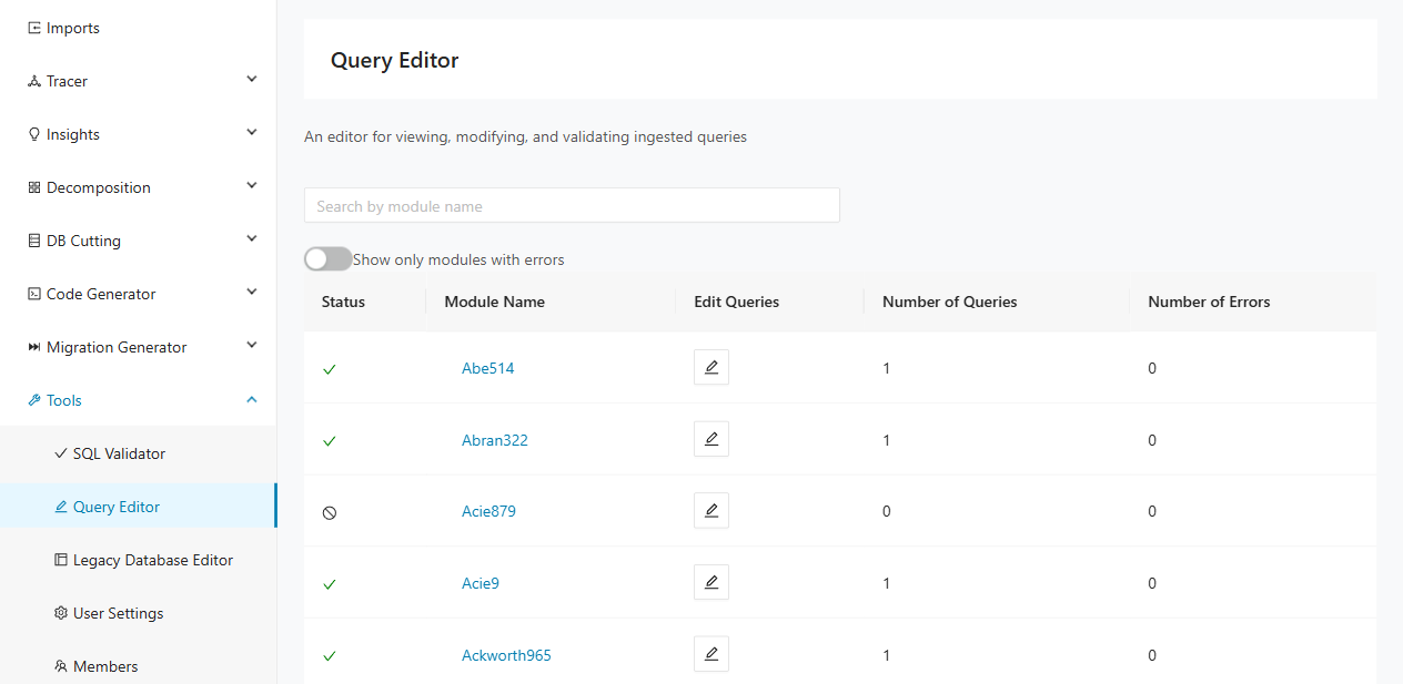
Module listing
The main view presents a table of all modules in the current project. Each row displays the module status, name, and query statistics.
| Column | Description |
|---|---|
| Status | A green checkmark indicates all queries parsed successfully. A red X indicates one or more queries have errors. A gray stop icon indicates the module has no queries. |
| Module Name | The name of the module. Click the name to highlight the row. |
| Edit Queries | Click the pencil icon to open the query editor for that module. |
| Number of Queries | The total number of queries associated with the module. |
| Number of Errors | The number of queries that failed to parse. |
Use the Search by module name text field to filter modules by name. Enable the Show only modules with errors toggle to display only modules that contain query parse errors.
The following screenshot shows the module listing with the error filter enabled, displaying only modules with parsing errors.
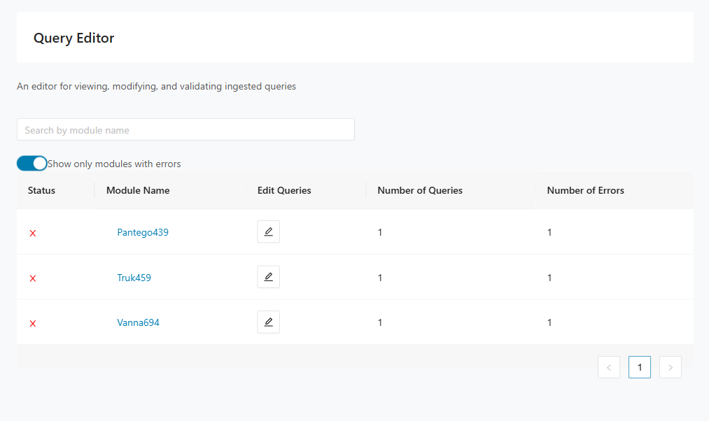
Editing queries for a module
Click the pencil icon in the Edit Queries column to open the query editor for a specific module. The heading updates to show the module name.
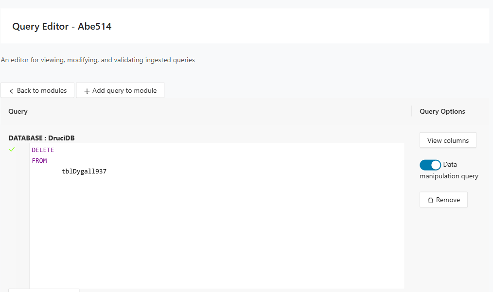
The query detail view contains the following elements:
- Back to modules — Click Back to modules to return to the module listing.
- Add query to module — Click Add query to module to create a new query for the module.
- Query table — Lists each query with two columns: Query and Query Options.
Each query row displays:
| Element | Description |
|---|---|
| Database label | The name of the database the query targets (for example, DATABASE : LegacyDB). |
| Query editor | An inline code editor with syntax highlighting and line numbers. SQL keywords are color-coded. You can edit the query text directly within this editor. |
| Submit for parsing | Click Submit for parsing to revalidate the query after making changes. |
| View columns | Click View columns to open the Add Table/Column dialog showing columns associated with the query. |
| Data manipulation query | A toggle that marks whether the query is a data manipulation query. |
| Remove | Click Remove to delete the query from the module. |
Queries with errors
When a query fails to parse, the editor displays a QUERY ERROR section below the query text. This section shows the full error message including the exception details and the location of the parsing failure.
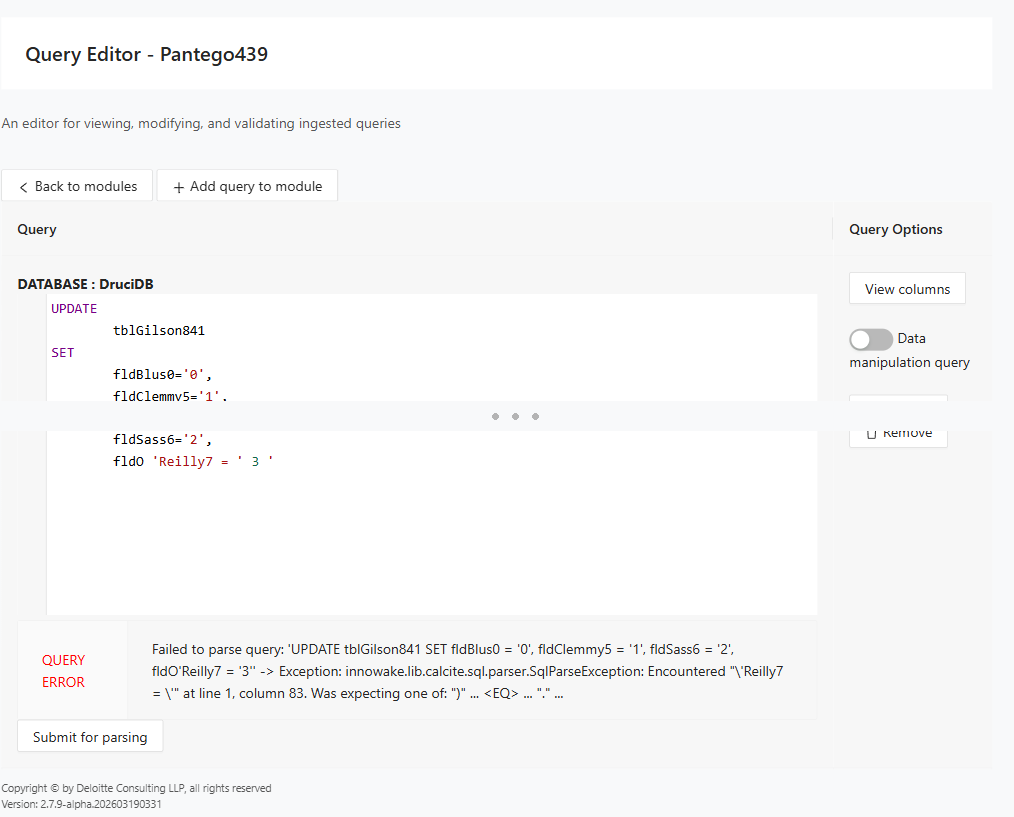
To fix a query error, edit the query text in the inline editor and click Submit for parsing to revalidate.
Viewing and managing columns
Click View columns on any query to open the Add Table/Column dialog. This dialog has two tabs: Current Columns and Add New Columns.
Current Columns
The Current Columns tab displays columns currently associated with the query.
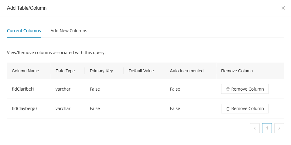
| Column | Description |
|---|---|
| Column Name | The name of the column. |
| Data Type | The data type of the column (for example, varchar). |
| Primary Key | Whether the column is a primary key. |
| Default Value | The default value assigned to the column, if any. |
| Auto Incremented | Whether the column auto-increments. |
| Remove Column | Click Remove Column to disassociate the column from the query. |
Pagination controls appear at the bottom of the table when there are multiple pages of columns.
Add New Columns
The Add New Columns tab allows you to associate new columns with the query.
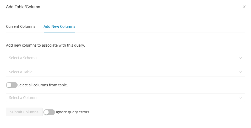
- Select a schema from the Select a Schema drop-down.
- Select a table from the Select a Table drop-down.
- Optionally, enable the Select all columns from table toggle to select every column in the chosen table.
- If not selecting all columns, choose a specific column from the Select a Column drop-down.
- Optionally, enable the Ignore query errors toggle to submit columns even if the query has parse errors.
- Click Submit Columns to associate the selected columns with the query.
Adding a new query
Click Add query to module to open the Create Query for Module dialog.
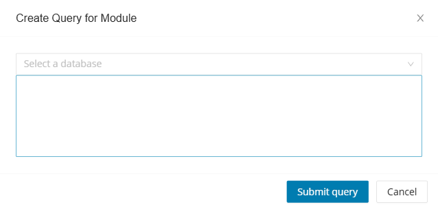
- Select the target database from the Select a database drop-down.
- Enter the SQL query text in the text area.
- Click Submit query to add the query to the module, or click Cancel to discard.
Legacy Database Editor
The Legacy Database Editor allows you to view and modify the imported database schema for your project. Use it as a repair tool to correct tables, columns, views, and other schema objects that are incorrect or outdated.
To access the Legacy Database Editor, select Tools > Legacy Database Editor in the left navigation panel.
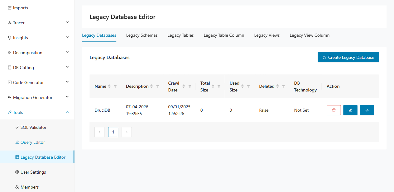
The editor organizes the schema into six tabs that follow the database hierarchy: databases, schemas, tables, table columns, views, and view columns. Each tab provides a table listing with sorting, filtering, pagination, and action buttons for creating, editing, and deleting entries. To navigate deeper into the hierarchy, click the arrow action button on a row. The next level opens, filtered to that parent object.
Legacy Databases
The Legacy Databases tab lists all databases in the current project.
| Column | Description |
|---|---|
| Name | The name of the database. |
| Description | A description or timestamp associated with the database. |
| Crawl Date | The date and time the database was last crawled. |
| Total Size | The total size of the database. |
| Used Size | The used size of the database. |
| Deleted | Whether the database is marked as deleted. |
| DB Technology | The database technology (for example, Postgres, MySQL, SQL Server, Oracle, or DB2). |
| Action | Provides options to delete, edit, or navigate into the database schemas. |
Each row in the Action column provides three buttons:
- Delete ( trash icon) — Remove the database entry.
- Edit ( pencil icon) — Open the Edit Legacy Database dialog to modify the database properties.
- Navigate (arrow icon) — Open the Legacy Schemas tab filtered to the selected database.
Creating a new legacy database
Click Create Legacy Database to open the New Legacy Database dialog.
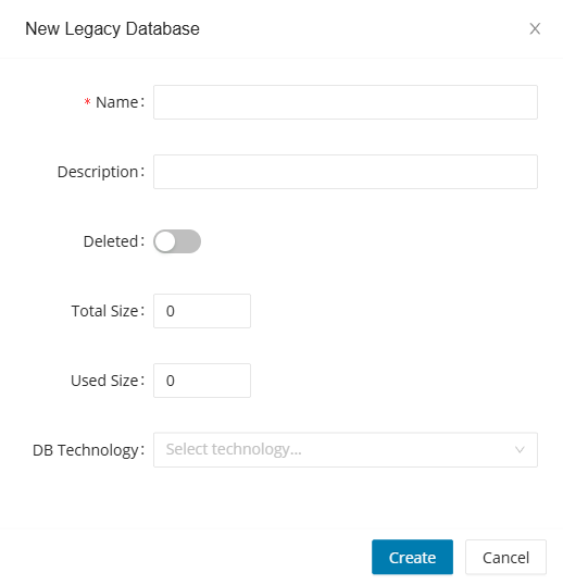
The dialog contains the following fields:
| Field | Description |
|---|---|
| Name | Required. The name of the database. |
| Description | An optional description for the database. |
| Deleted | A toggle to mark the database as deleted. |
| Total Size | The total size of the database (numeric input). |
| Used Size | The used size of the database (numeric input). |
| DB Technology | Select the database technology from the drop-down. Options include Postgres, MySQL, SQL Server, Oracle, and DB2. |
Click Create to add the database, or click Cancel to discard.
Editing a legacy database
Click the pencil icon in the Action column to open the Edit Legacy Database dialog. This dialog contains the same fields as the creation dialog, pre-populated with the existing values. Click Update to save changes.
Legacy Schemas
The Legacy Schemas tab displays the schemas belonging to a selected database. The heading shows the parent database name (for example, Legacy Schemas ( LegacyDB )).
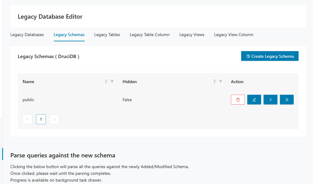
| Column | Description |
|---|---|
| Name | The name of the schema. |
| Hidden | Whether the schema is hidden from the decomposition views. |
| Action | Provides options to delete, edit, navigate to tables, or navigate to views. |
Each row in the Action column provides four buttons:
- Delete ( trash icon) — Remove the schema.
- Edit ( pencil icon) — Open the edit dialog to modify the schema.
- Navigate to tables (arrow icon) — Open the Legacy Tables tab filtered to the selected schema.
- Navigate to views (double arrow icon) — Open the Legacy Views tab filtered to the selected schema.
Click Create Legacy Schema to add a new schema to the database.
Below the schema table, the Parse queries against the new schema section reparses all queries against schema modifications. Click Parse to start the process. Progress is available in the background task drawer.
Legacy Tables
The Legacy Tables tab lists all tables within a selected schema. The heading shows the parent schema name (for example, Legacy Tables ( public )).
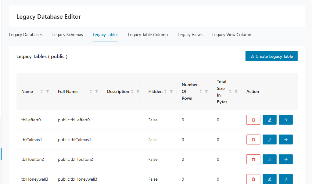
| Column | Description |
|---|---|
| Name | The name of the table. |
| Full Name | The fully qualified name including the schema (for example, public.customers). |
| Description | An optional description of the table. |
| Hidden | Whether the table is hidden from the decomposition views. |
| Number Of Rows | The number of rows in the table. |
| Total Size In Bytes | The total size of the table in bytes. |
| Action | Provides options to delete, edit, or navigate to the table columns. |
Click Create Legacy Table to add a new table to the schema.
Legacy Table Column
The Legacy Table Column tab displays all columns for a selected table. The heading shows the parent table name (for example, Legacy Table Columns ( customers )).
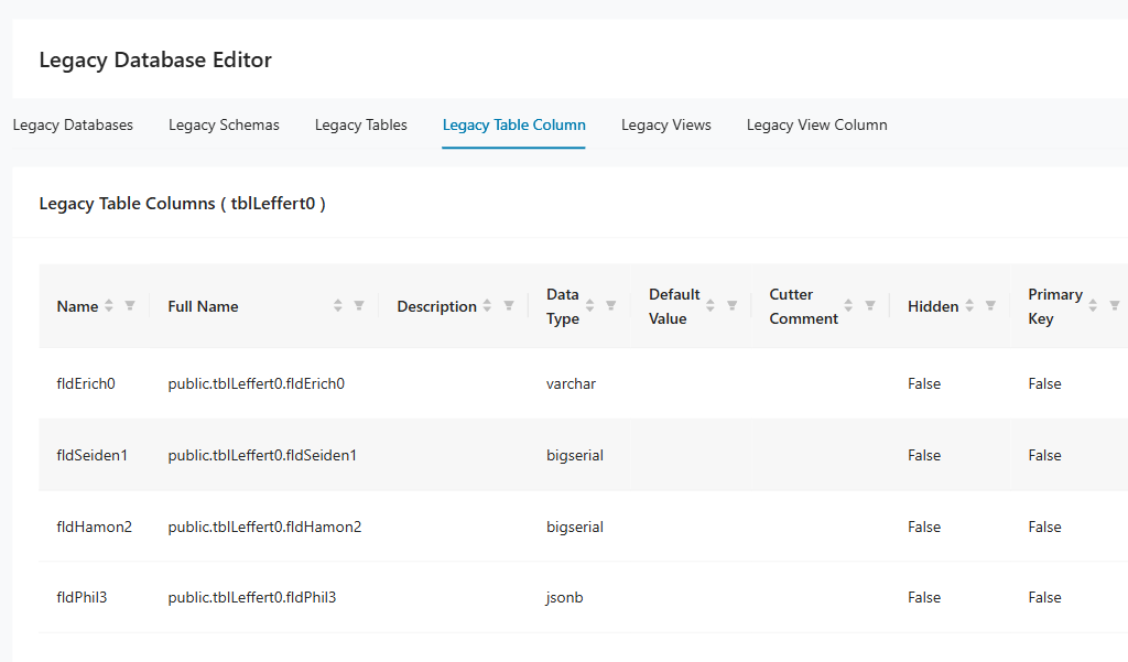
| Column | Description |
|---|---|
| Name | The name of the column. |
| Full Name | The fully qualified name including the schema and table (for example, public.customers.email). |
| Description | An optional description of the column. |
| Data Type | The data type of the column (for example, varchar, bigserial, jsonb). |
| Default Value | The default value assigned to the column, if any. |
| Cutter Comment | A comment field used by the decomposition engine. |
| Hidden | Whether the column is hidden from the decomposition views. |
| Primary Key | Whether the column is a primary key. |
| Auto Incremented | Whether the column auto-increments. |
| Action | Provides options to delete or edit the column. |
Click Create Legacy Table Column to add a new column to the table.
Legacy Views
The Legacy Views tab lists all views within a selected schema. The heading shows the parent schema name (for example, Legacy Views ( public )).
| Column | Description |
|---|---|
| Name | The name of the view. |
| Hidden | Whether the view is hidden from the decomposition views. |
| Action | Provides options to delete, edit, or navigate to the view columns. |
Click Create Legacy View to add a new view to the schema.
Legacy View Column
The Legacy View Column tab displays all columns for a selected view. The heading shows the parent view name, or prompts you to select a view if none is selected.
| Column | Description |
|---|---|
| Name | The name of the view column. |
| Hidden | Whether the column is hidden. |
| Column Name | The name of the underlying column. |
| Action | Provides options to delete or edit the view column. |
Click Create Legacy View Column to add a new column to the view. This button is disabled until you select a view.
User Settings
User Settings allows you to configure graph display preferences for the various graph views in Decompose. These settings control layout algorithms, subgraph expansion behavior, caching, and filtering options for the Legacy Database, Query Paths, and Migration Report graphs.
To access the User Settings, select Tools > User Settings in the left navigation panel.
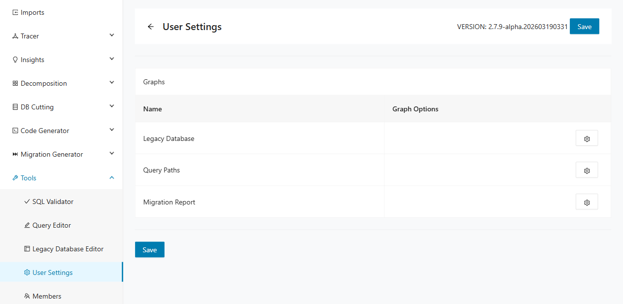
The page displays a Graphs section containing a table with two columns:
| Column | Description |
|---|---|
| Name | The name of the graph view. |
| Graph Options | Click the settings icon to open the Graph Options dialog for that graph. |
The three configurable graphs are:
- Legacy Database — controls the database schema graph in the decomposition views;
- Query Paths — controls the graph that visualizes module and query relationships;
- Migration Report — controls the graph displayed in migration reports.
Click Save at the top or bottom of the page to persist any changes you make to the graph options.
Graph Options
Click the settings icon in the Graph Options column for any graph to open its Graph Options dialog. Each dialog contains settings organized into sections: Display Style, Subgraph Expansion, Caching, and Filtering. The available settings vary by graph view.
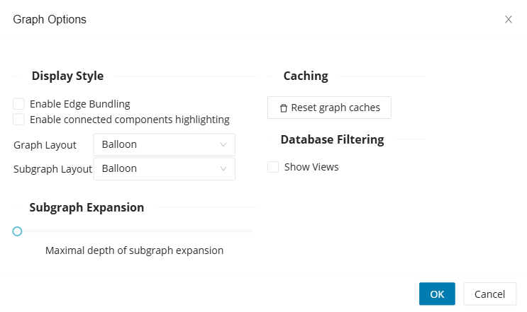
The following table lists all configurable settings across the three graph views.
| Section | Setting | Description | Graph View |
|---|---|---|---|
| Display Style | Enable Edge Bundling | Groups graph edges together to reduce visual clutter. | All |
| Enable connected components highlighting | Highlights connected components in the graph with distinct colors. | All | |
| Graph Layout | Sets the layout algorithm for the main graph. Options: Balloon, Hierarchical, Organic, Radial. | All | |
| Subgraph Layout | Sets the layout algorithm for subgraphs. Options: Balloon, Hierarchical, Organic, Radial. | All | |
| Subgraph Expansion | Maximal depth of subgraph expansion | Controls how many levels deep subgraphs are expanded automatically. | Legacy Database |
| Fully expand bounded contexts in subgraph | Automatically expands all bounded contexts when viewing a subgraph. | Query Paths, Migration Report | |
| Fully expand modules in subgraph | Automatically expands all modules when viewing a subgraph. | Query Paths, Migration Report | |
| Maximal depth of module hierarchy | Controls how many levels deep the module hierarchy is expanded. | Query Paths, Migration Report | |
| Caching | Reset graph caches | Clears all cached graph data. Use this after making schema or decomposition changes that are not yet reflected in the graph. | All |
| Filtering | Show Views | Includes database views in the graph when enabled. | Legacy Database |
| Has Query | Filters the graph to show only modules that have at least one query. | Query Paths | |
| Has ReadQuery | Filters the graph to show only modules that have at least one read query. | Query Paths | |
| Has WriteQuery | Filters the graph to show only modules that have at least one write query. | Query Paths |
Click OK to apply the settings, or click Cancel to discard changes.
Members
The Members subpage is a user management area that allows you to manage user access to clients and projects. You can create new users, assign user roles, and grant access to specific clients and their associated projects. To navigate to the Members subpage, select Tools > Members.
The page lists each client as a collapsible accordion panel. Expand a client to manage its members. Each panel contains two sub-tabs: Managers and Project Members.
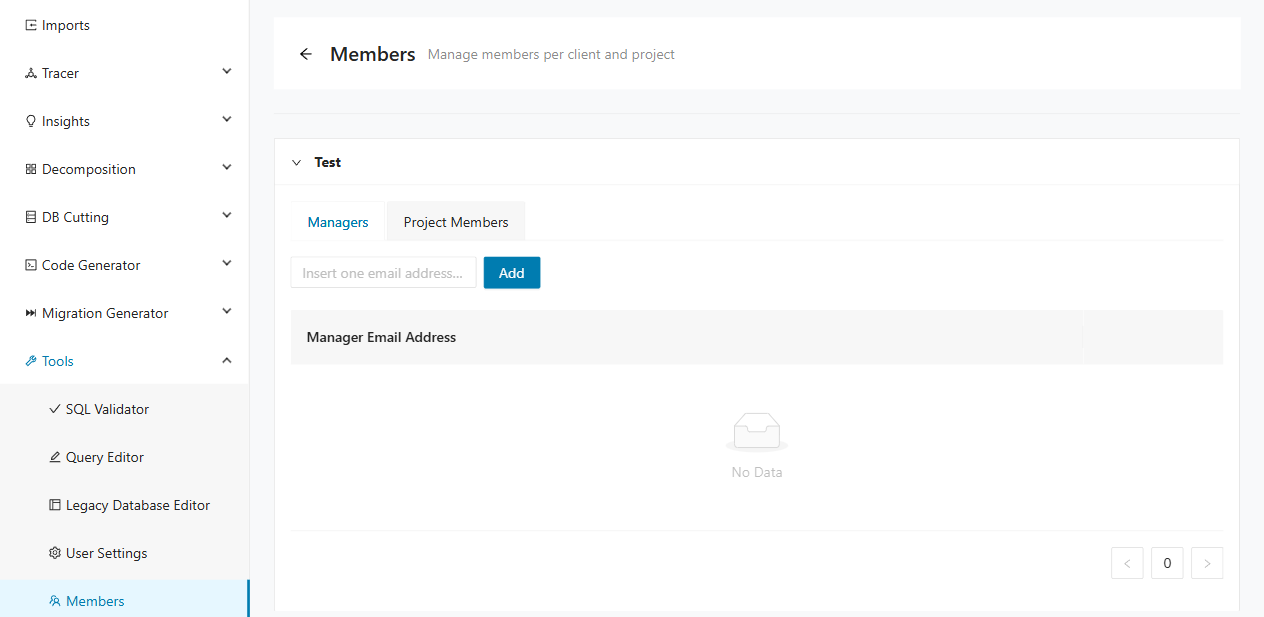
| Sub-tab | Description |
|---|---|
| Managers | Users with the Manager role are added on this tab. Managers have elevated access to the client and its associated projects. |
| Project Members | Users with Editor or Viewer roles are added on this tab. Users are assigned to specific projects with a role that defines their access rights. |
Creating a new manager role
Each user is identified by a unique email address. To assign the Manager role to a user:
- Expand the target client panel.
- Select the Managers tab.
- Enter the user's email address in the input field.
- Click Add .
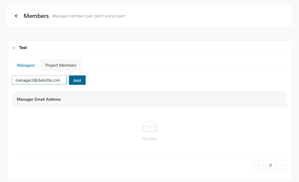
The system adds the manager under the respective client, granting access to that client and its associated projects. The Manager Email Address table lists all current managers. Each row includes a delete icon to remove a manager.
Creating a new project member
To create a new project member:
- Expand the target client panel.
- Select the Project Members tab.
- Enter the user's email address in the Email field.
- Open the Project drop-down and select one or more projects to assign the user to.
- Under Role, select either Viewer or Editor.
- Click Add .
The following screenshot shows the Project Members tab with the add-member form and the projects table.
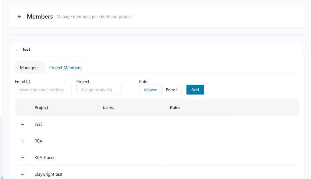
The projects table lists all projects belonging to the client. Expand a project row to view the User Email and User Role columns for members assigned to that project.
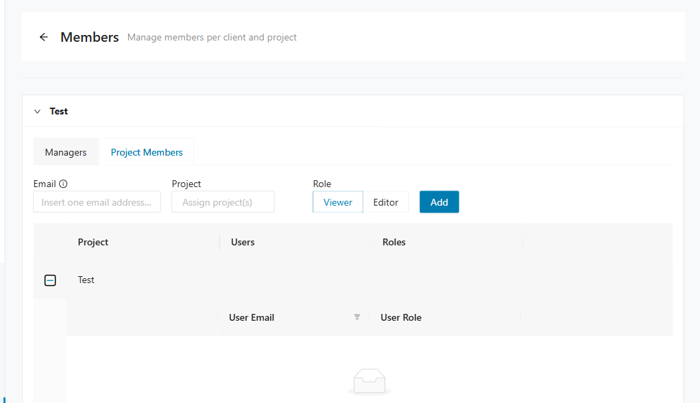
Changing user roles or deleting users
You can change user roles — for example, from Editor to Viewer — which automatically adjusts the permissions. You can also delete users.
To change a user's role, expand the project row to reveal the member list, then select a new role from the User Role drop-down for that user. To delete a user, click the delete icon in the corresponding row.
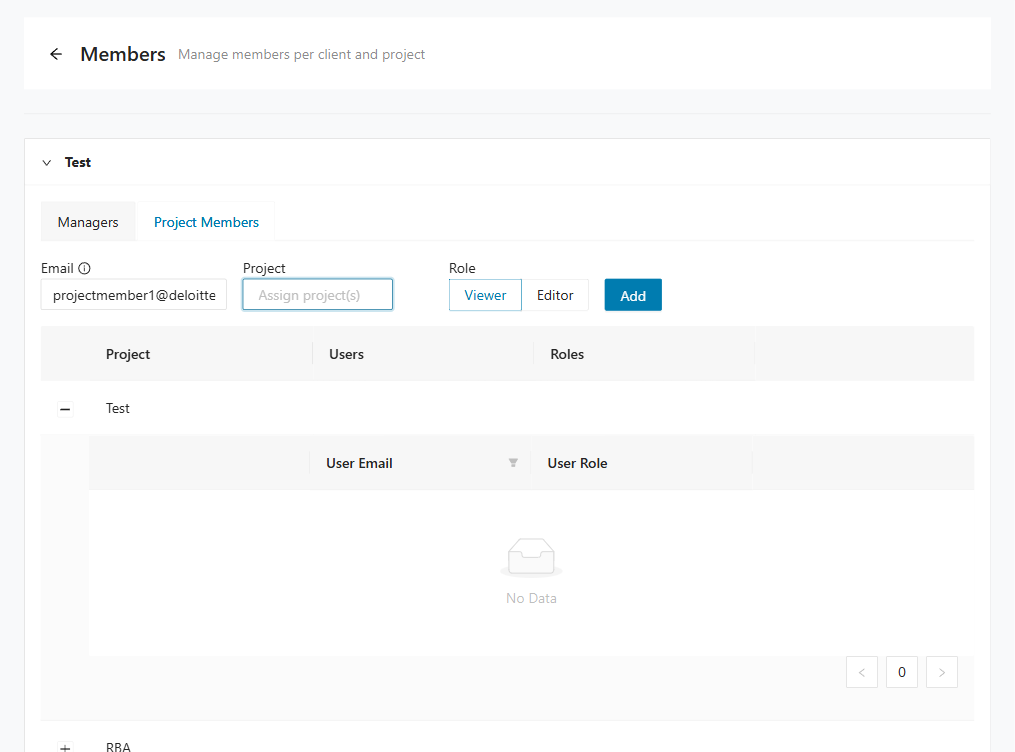
Permissions overview table
Decompose uses four user roles to control access to clients, projects, and administrative functions. The table below summarizes the permissions linked to each role.
| Area | Action | Admin | Manager | Editor | Viewer |
|---|---|---|---|---|---|
| Access to Members subpage | ✅ | ✅ | ❌ | ❌ | |
| Projects | Access to all projects | ✅ | ❌ | ❌ | ❌ |
| Access to projects to which access was granted | ✅ | ✅ | ✅ | ✅(read-only) | |
| Create new projects | ✅ | ✅ | ❌ | ❌ | |
| Duplicate or delete projects | ✅ | ✅ | ❌ | ❌ | |
| Edit or modify projects | ✅ | ✅ | ✅ | ❌ | |
| View or export reports | ✅ | ✅ | ✅ | ✅ | |
| Import or upload files and data | ✅ | ✅ | ✅ | ❌ | |
| Clients | Access to all clients | ✅ | ❌ | ❌ | ❌ |
| Access to clients to which access was granted | ✅ | ✅ | ✅ | ✅(read-only) | |
| Create or delete clients | ✅ | ❌ | ❌ | ❌ | |
| User Management | Manage users and organize access to all clients and projects | ✅ | ❌ | ❌ | ❌ |
| Manage users and organize access to specific clients and projects | ✅ | ✅ | ❌ | ❌ | |
| Create or delete Manager roles | ✅ | ❌ | ❌ | ❌ | |
| Create or delete project members, assign them to user roles and to client-related projects | ✅ | ❌ | ❌ | ❌ | |
| Edit user role of existing project members | ✅ | ✅ | ❌ | ❌ | |
| Add or remove Viewers or Editors to or from clients or projects | ✅ | ✅ | ❌ | ❌ |
Role descriptions:
- Viewer — Read-only access to assigned clients and projects. A Viewer can view and export reports but cannot upload, import, or modify data.
- Editor — Access to assigned clients and projects with the ability to edit projects and import data. An Editor cannot create, duplicate, or delete projects, nor access the Members subpage.
- Manager — Access to the Members subpage and all Editor permissions. A Manager can also create, duplicate, or delete projects and manage user access. Managers can only access explicitly assigned clients and projects.
- Admin — Full access to Decompose. An Admin can manage all clients, projects, users, and roles across the platform.
Tracer
Tracer
Tracer helps you use runtime evidence to understand how users move through a legacy application. It combines traced users, taxonomy mappings, uploaded logs, and module usage so you can identify candidate domains and focus later decomposition work.
Tracer workflow
The Tracer workflow is easiest to follow when you move from concepts, to master data, to log ingestion, and finally to reports. Each step builds on the previous one, so missing setup in an earlier page usually affects downstream analysis results. Use the sequence below as the recommended order for onboarding a new project into Tracer.
Use Tracer in this order:
- Review About Tracer to understand the tracing model, instrumentation options, and analysis approach.
- Add or import Traced Users.
- Create, merge, or import entries in Taxonomy Selection.
- Create the mappings in Taxonomy User Mapping.
- Upload runtime, database query, or OpenTelemetry logs on Upload Logfile.
- Review Mining Modules and the Tracer Reports to understand usage patterns and taxonomy probabilities.
About Tracer
The conceptual overview for Tracer now lives on the dedicated About Tracer page. The page explains the Tracer model, application overview, data gathering, instrumentation, OpenTelemetry, and data analysis topics in more detail. Start there if you need the background behind the runtime evidence and probability calculations used elsewhere in this section.
Traced users
The Traced Users page stores the users or actors that Tracer associates with runtime activity. These entries are foundational because Tracer uses them to connect observed system behavior to business-facing user groups. Maintain this page before loading logs so the resulting activity can be mapped meaningfully.
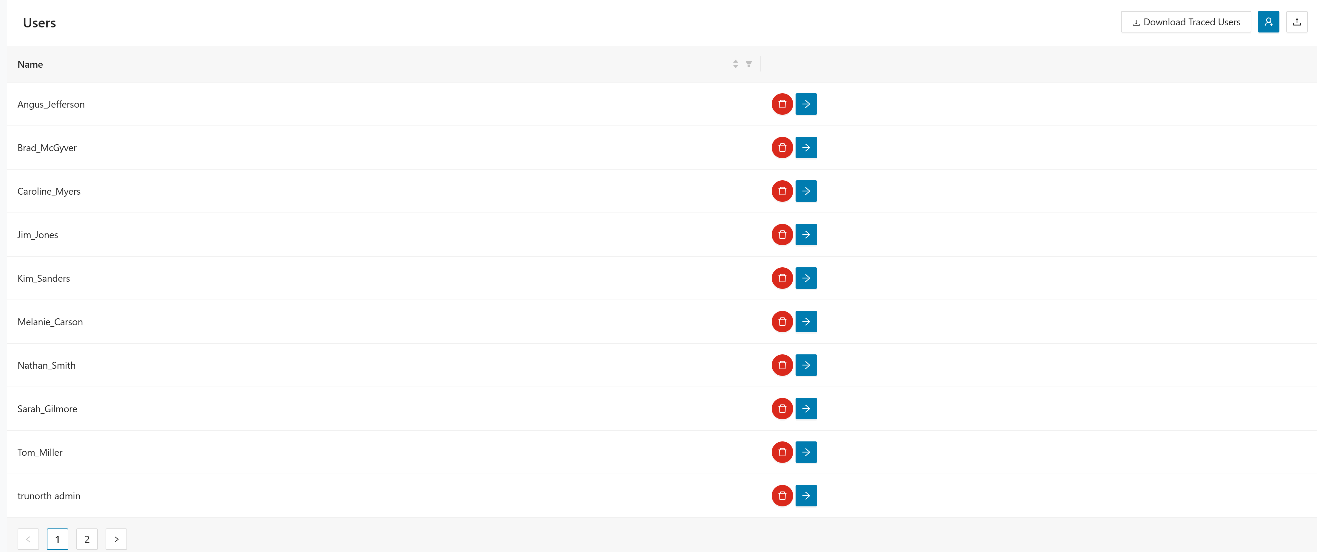
The page accepts CSV uploads.
Use the controls in the upper-right corner of the page to work with traced users:
- Click Download Traced Users to export the current user list.
- Click to create a traced user manually.
- Click to import users from a file.
Managing traced users
Use these actions to create and maintain traced users.
- Click .
- Enter the value in User name.
- Click
to create the user and return to the user list.

- Click to delete the user. The application asks for confirmation before the delete is applied.
- Click to open User Identities for the selected user.
- Maintain the identities associated with that traced user on the User Identities page.
Taxonomy selection
Use Taxonomy Selection to maintain the business taxonomies that Tracer uses during analysis. These taxonomies represent the candidate business domains that Tracer will compare against runtime behavior. Define them carefully so the later probabilities align with the business structure you want to evaluate.
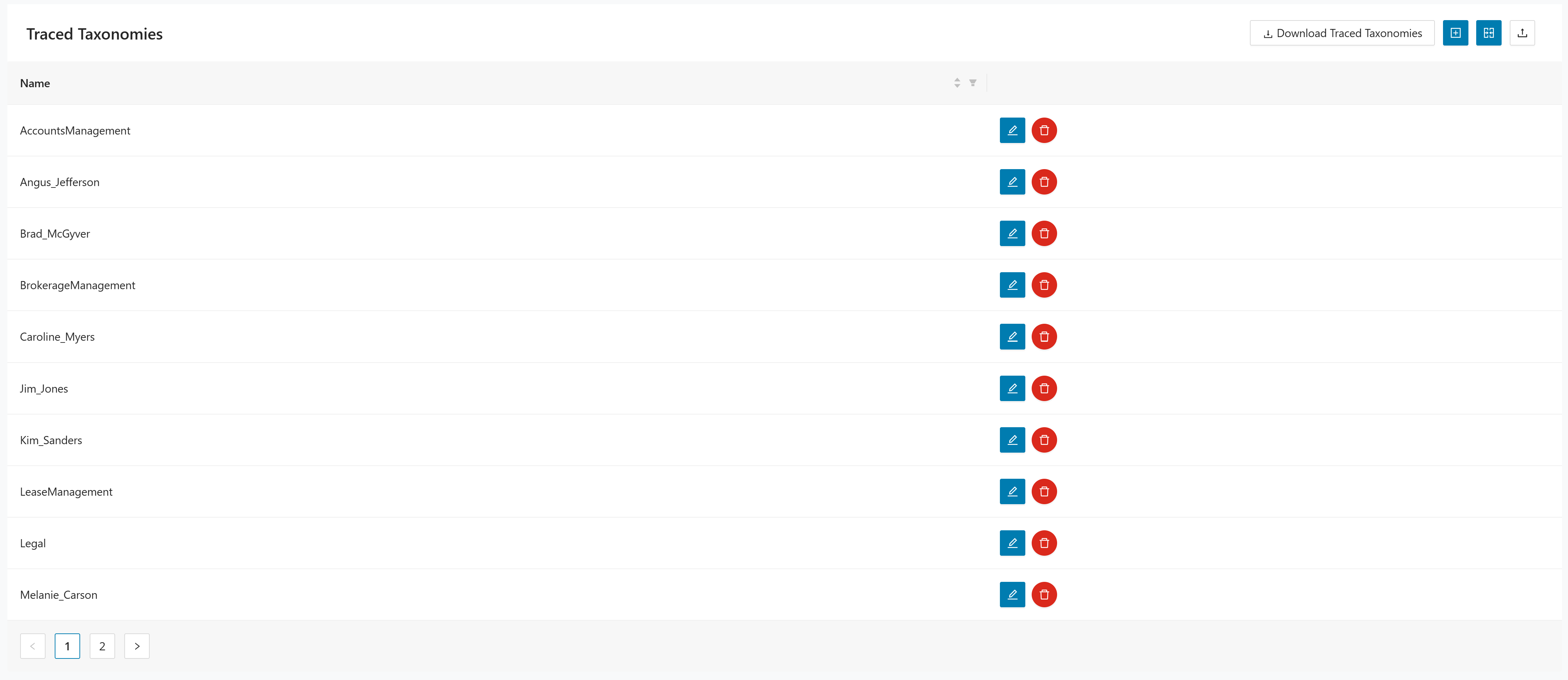
The page accepts CSV uploads.
The toolbar provides the following actions:
- Click Download Traced Taxonomies to export the current taxonomy list.
- Click to create a taxonomy manually.
- Click to combine two taxonomy entries.
- Click to import taxonomy data.
Managing taxonomies
Use these actions to create, merge, and maintain taxonomy entries.
- Click .
- Enter the value in Taxonomy Name.
- Click
to create the taxonomy and return to the taxonomy list.

- Click .
- Select the target taxonomy in Taxonomy to merge into.
- Select the source taxonomy in Taxonomy to be merged from.
- Click
to merge the selected taxonomies.
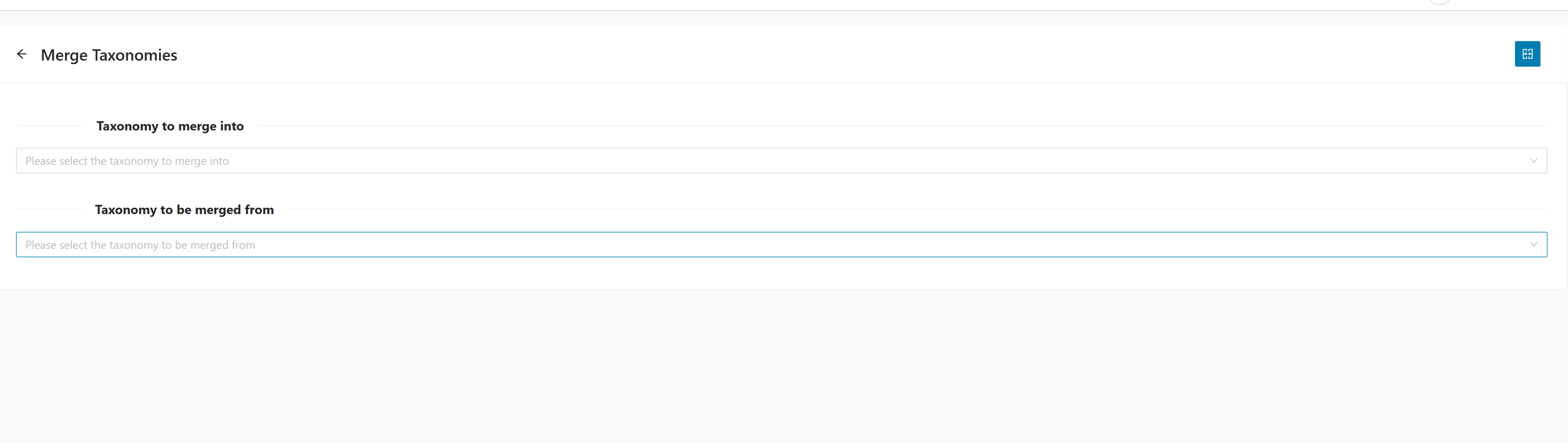
- Click to open Edit Taxonomy. The page prepopulates Taxonomy Name for the selected entry.
- Update the taxonomy name and click to apply the change.
- Click to delete the taxonomy. The application asks for confirmation before the delete is applied.
Taxonomy user mapping
Use Taxonomy User Mapping to connect users to the taxonomy they represent. Tracer depends on this mapping to turn raw user activity into module-to-taxonomy probabilities. Keep it accurate because incorrect mappings can distort the analysis results significantly.
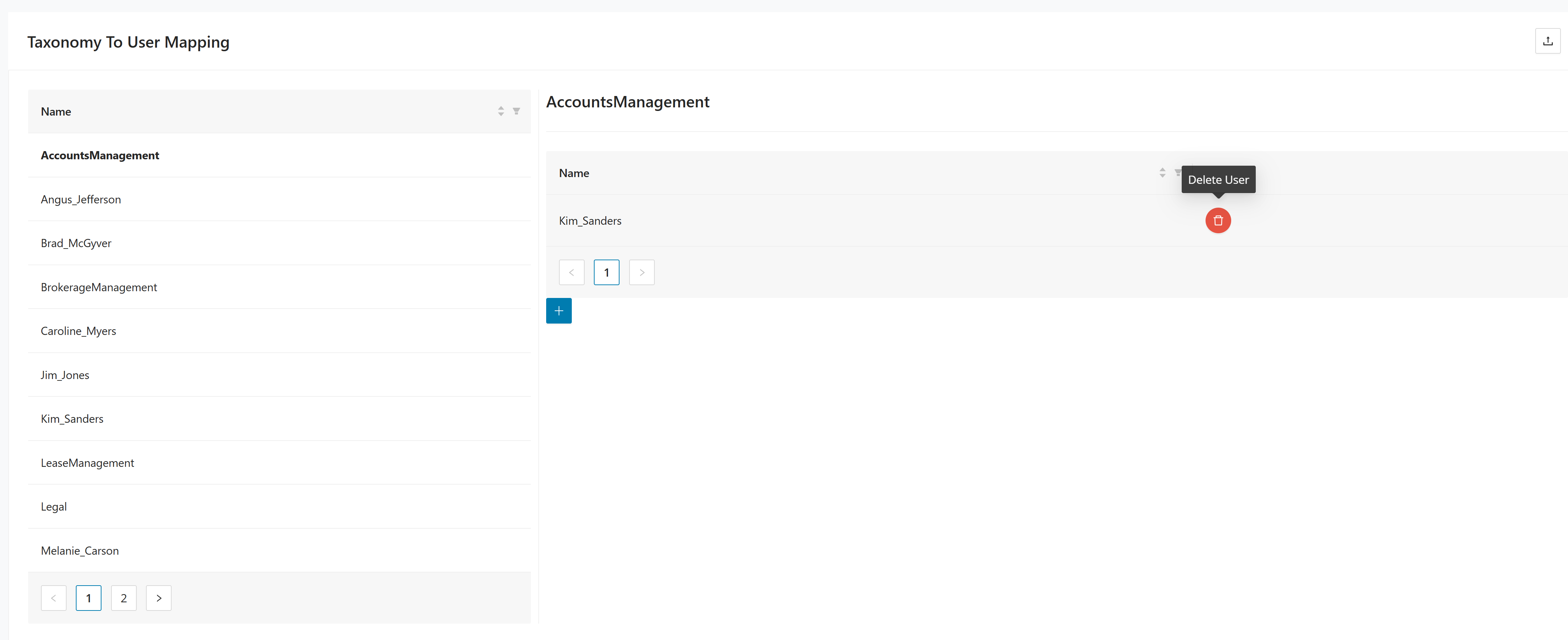
Use a CSV file when you import mappings on this page. A valid file uses the headers UserName;TaxonomyName.
The page is split into two lists:
- The left side shows available taxonomies.
- The right side shows the users mapped to the selected taxonomy.
Use the controls on this page as follows:
- Select a taxonomy from the list on the left.
- Review the mapped users for the selected taxonomy in the right panel.
- Click Add mapped users for the selected taxonomy to open Create Taxonomy To User Mapping.
- Select the user from the dropdown to map on the creation page and click to add the mapping.
- Click near the page title to import mapping data from a CSV file.
The Add mapped users action is context-sensitive. It works on the taxonomy that is currently selected in the left panel and opens a dedicated mapping page for that taxonomy.
Managing taxonomy user mappings
Use these actions to add, import, and remove taxonomy user mappings.
- Select a taxonomy from the list on the left.
- Click Add mapped users for the selected taxonomy.
- Select the user to map on the creation page.
- Click
to add the mapping.

- Click near the page title.
- Select a CSV file that uses the headers
UserName;TaxonomyName. - Complete the import to load the mappings into the page.
- Select a taxonomy from the list on the left.
- Review the mapped users in the right panel.
- Click in the mapped-users table to remove the selected user from that taxonomy.
Mining modules
The Mining Modules page lists the modules discovered by tracing and shows the module metadata available for later reporting and decomposition. It gives you a direct view of the technical artifacts Tracer has identified from the collected evidence. Use it to confirm coverage, inspect module details, and control inclusion in later results.
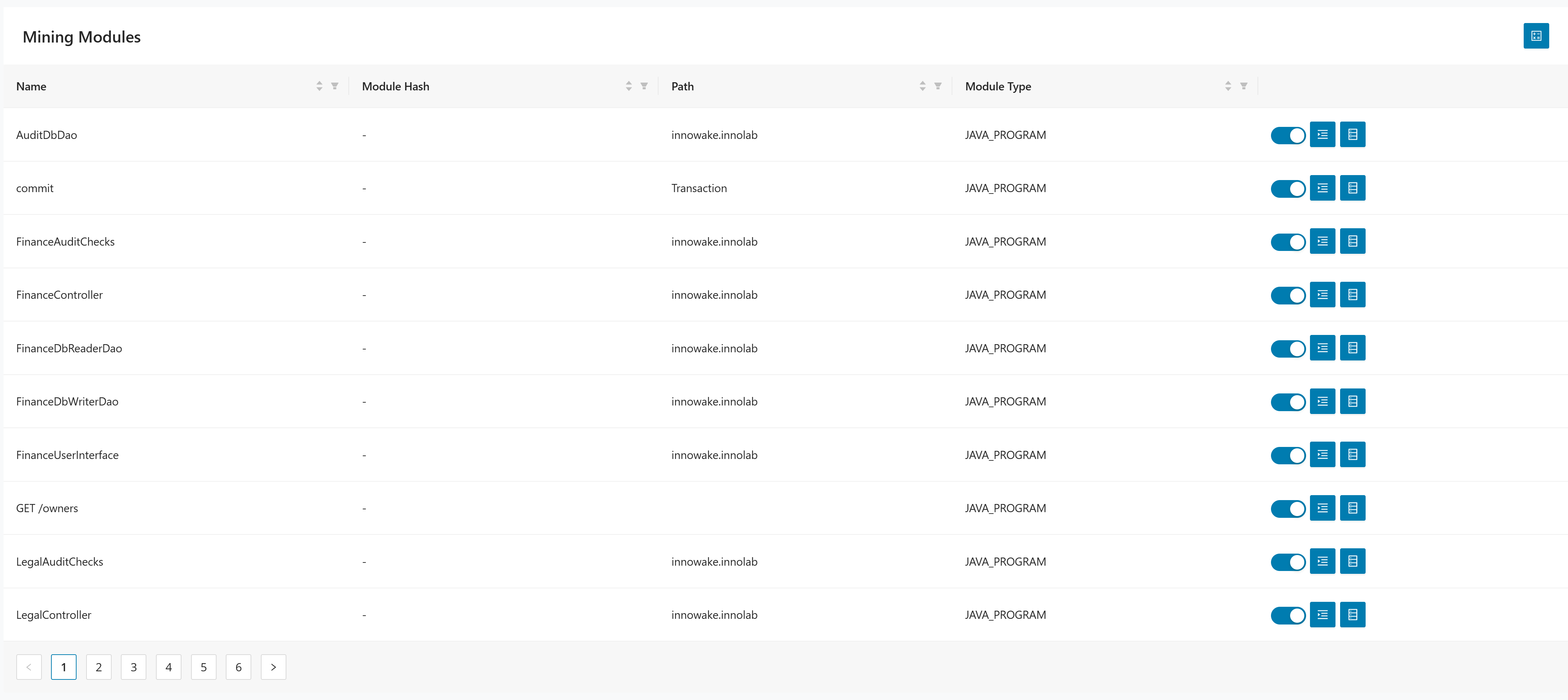
The table includes these columns:
- Name identifies the module.
- Module Hash shows the unique technical identifier for the module.
- Path shows the source or logical path when available.
- Module Type identifies the type of module, such as
EXEC_PGM,FILE,PROC, orSUBROUTINE.
Using mining module actions
Use these actions to include modules in results and review related details.
- Use the switch in the module row to control whether the module is included in Tracer results.
- Use toggle on to include the module in results.
- Use
toggle off to exclude the module from results.
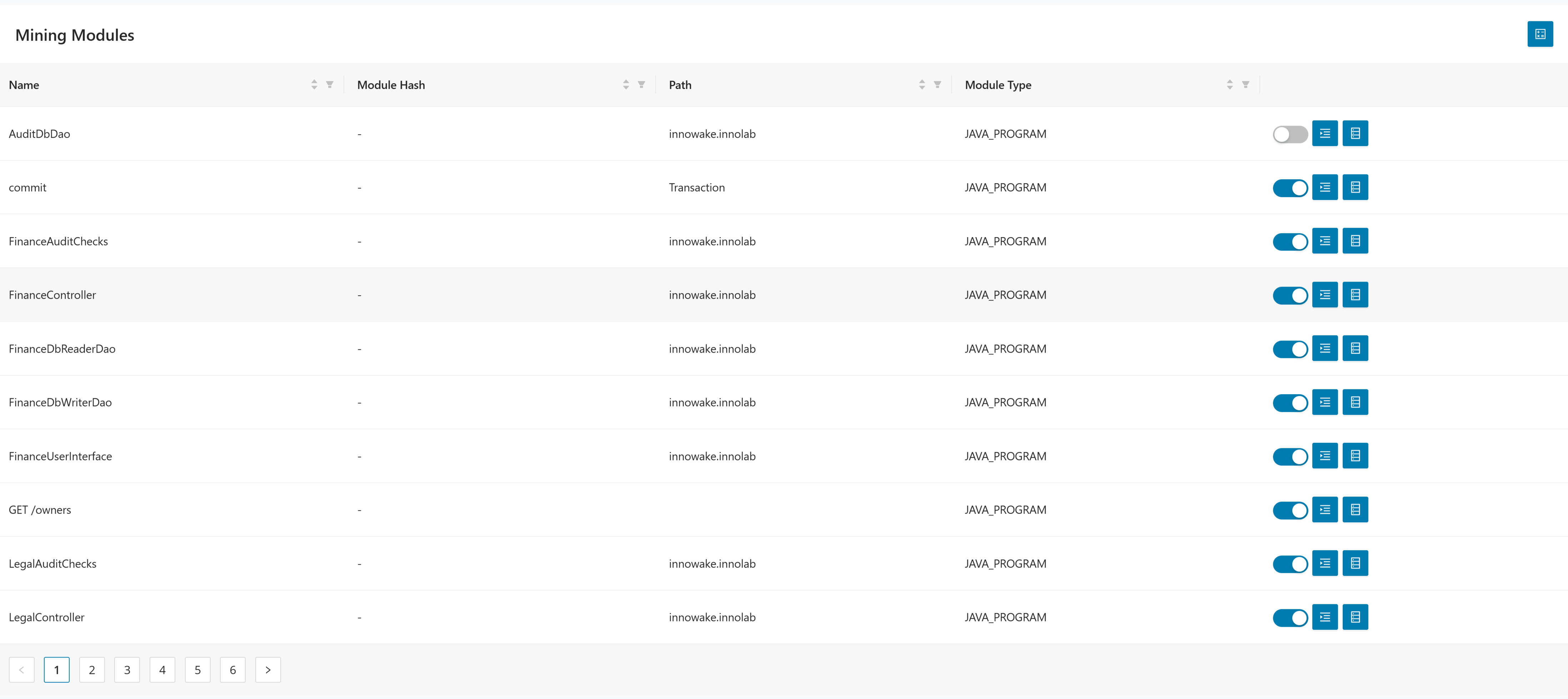
- Click Mining Functions to review the functions for the selected module.
- Review the traced functions for that module.
- Use the recorded line range and duration values to inspect the function activity.

- Click Database Queries to review the database queries for the selected module.
- Review the traced SQL statements associated with that module.
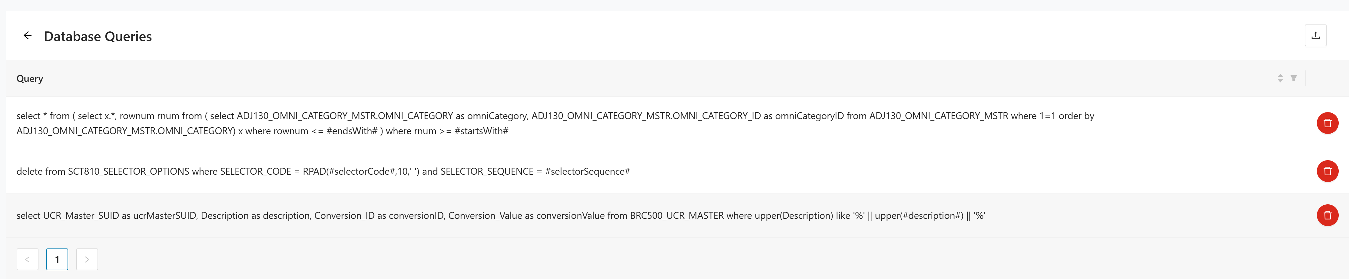
Use the pagination controls at the bottom of the table to move through the full module list.
Upload logfile
Use Upload Logfile to import trace data into the project. This is the step where runtime evidence enters Tracer and becomes available for processing and probability calculations. Use the correct upload panel for each log type so the collector can interpret the data properly.
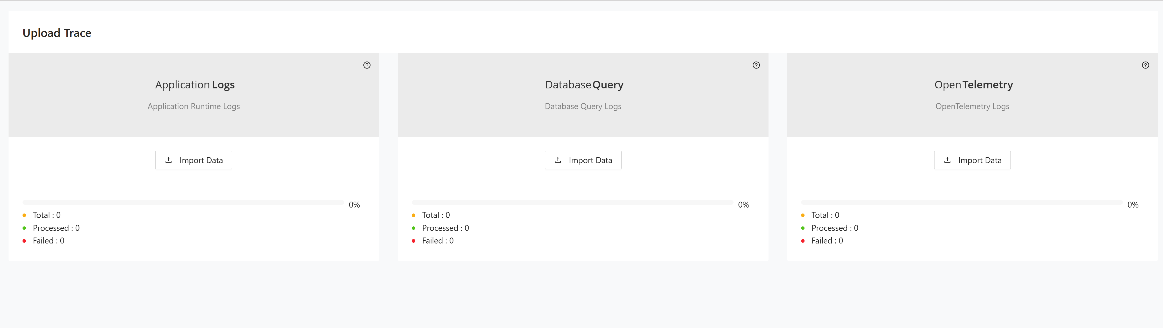
The page contains three upload panels:
- Application Runtime Logs for application runtime traces.
- Database Query Logs for database access traces.
- OpenTelemetry Logs for trace data produced by OpenTelemetry instrumentation.
Uploading logs
Use the appropriate panel to load each log type into Tracer.
- In Application Runtime Logs, click Import Data.
- Select the runtime log file to upload.
- Monitor the progress bar and the counters for Total, Processed, and Failed.
- In Database Query Logs, click Import Data.
- Select the database query log file to upload.
- Monitor the progress bar and the counters for Total, Processed, and Failed.
- In OpenTelemetry Logs, click Import Data.
- Select the OpenTelemetry log file to upload.
- Monitor the progress bar and the counters for Total, Processed, and Failed.
Repeat these steps for each log type you want to load.
Reports
The Reports section exposes the analysis outputs generated from the traced users, taxonomies, mappings, and uploaded logs. These views help you turn collected runtime data into decisions about usage, taxonomy alignment, and decomposition candidates. Review them after the upstream setup and log-ingestion steps are complete.
Results dashboard
The Results Dashboard provides download links for the main Tracer output files and summarizes module usage.
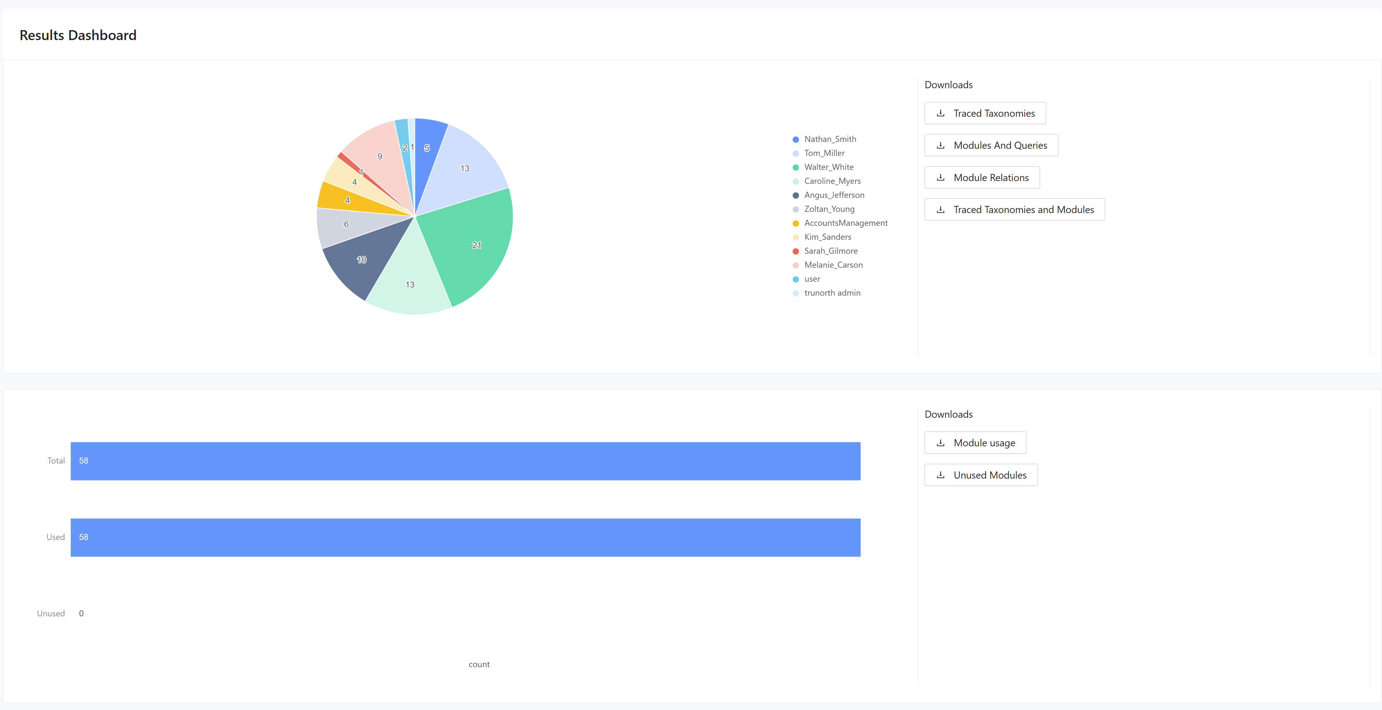
Use the dashboard to download:
- Traced Taxonomies
- Modules And Queries
- Module Relations
- Traced Taxonomies and Modules
- Module usage
- Unused Modules
The chart in the lower section compares the used and unused module counts for the project.
Taxonomy usage
The Taxonomy Usage report calculates the probability that modules belong to a taxonomy based on traced activity.
For the calculation model and worked examples behind these probability values, see Tracer Probability Calculation.
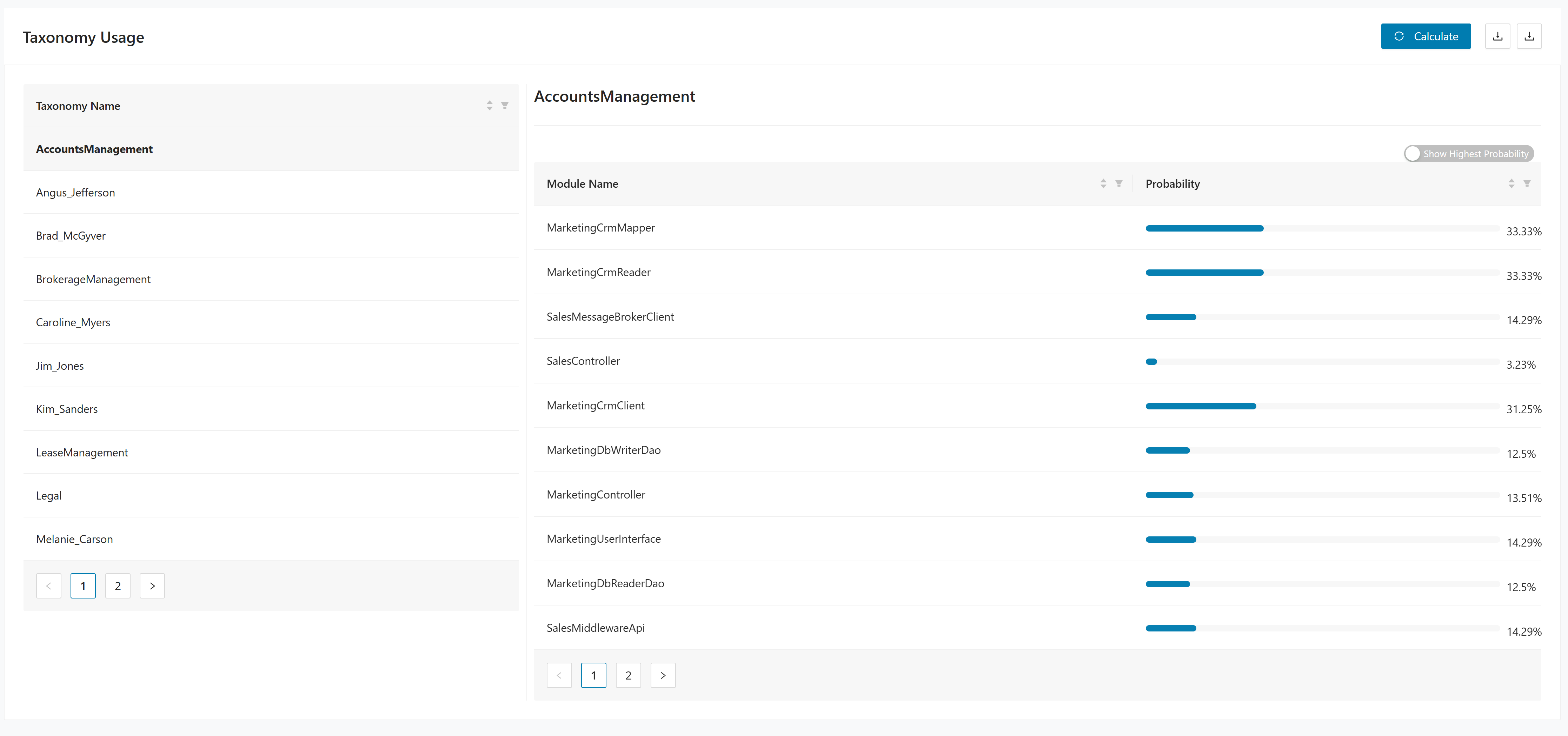
Use this page as follows:
- Click Calculate to run the probability analysis.
- Review the taxonomy list in the first table.
- Use Show Highest Probability to focus on the strongest taxonomy matches for modules.
Module usage
The Module Usage report combines the traced module list with usage counts by taxonomy.
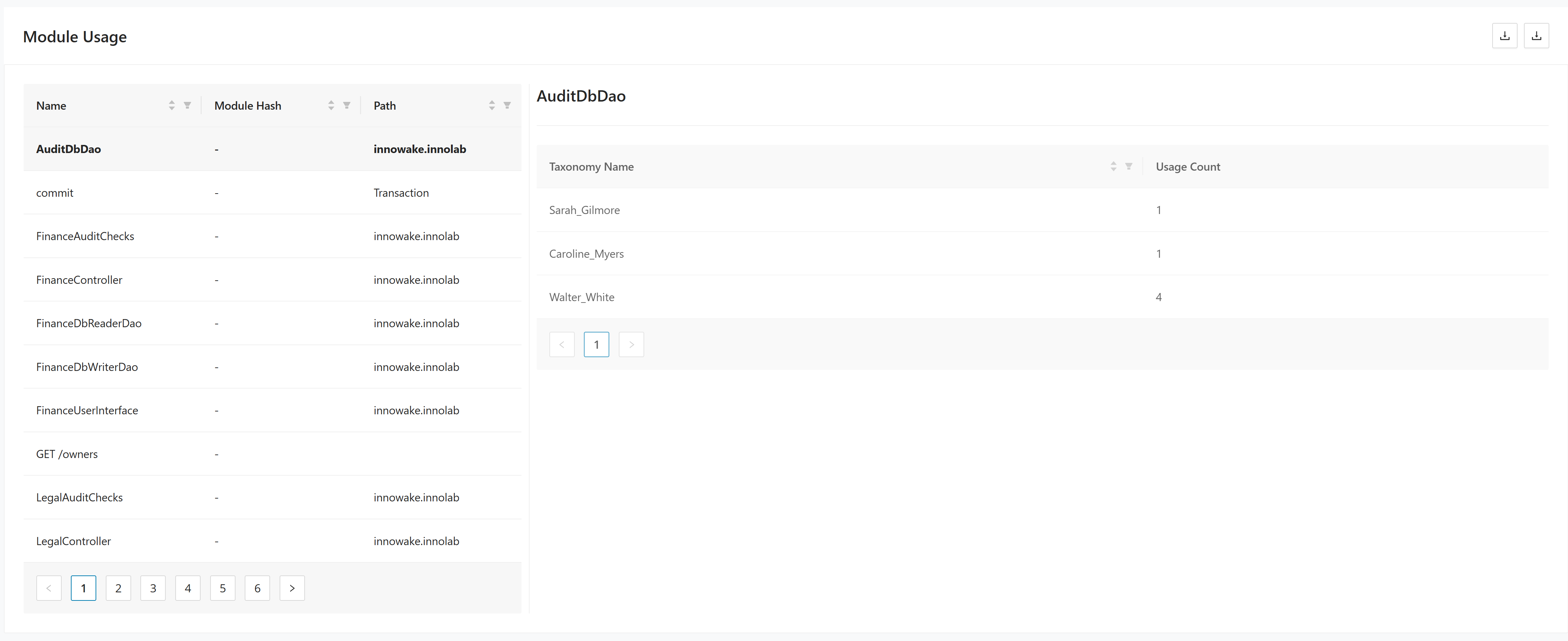
Use this page as follows:
- Review the upper table for the traced module list, including the module name, hash, and path.
- Review the lower table for the usage count per taxonomy when probability results are available.
- Use the pagination controls to move through the module list.
Total function usage
The Total Function Usage report lists functions together with their taxonomy, module, and probability values.
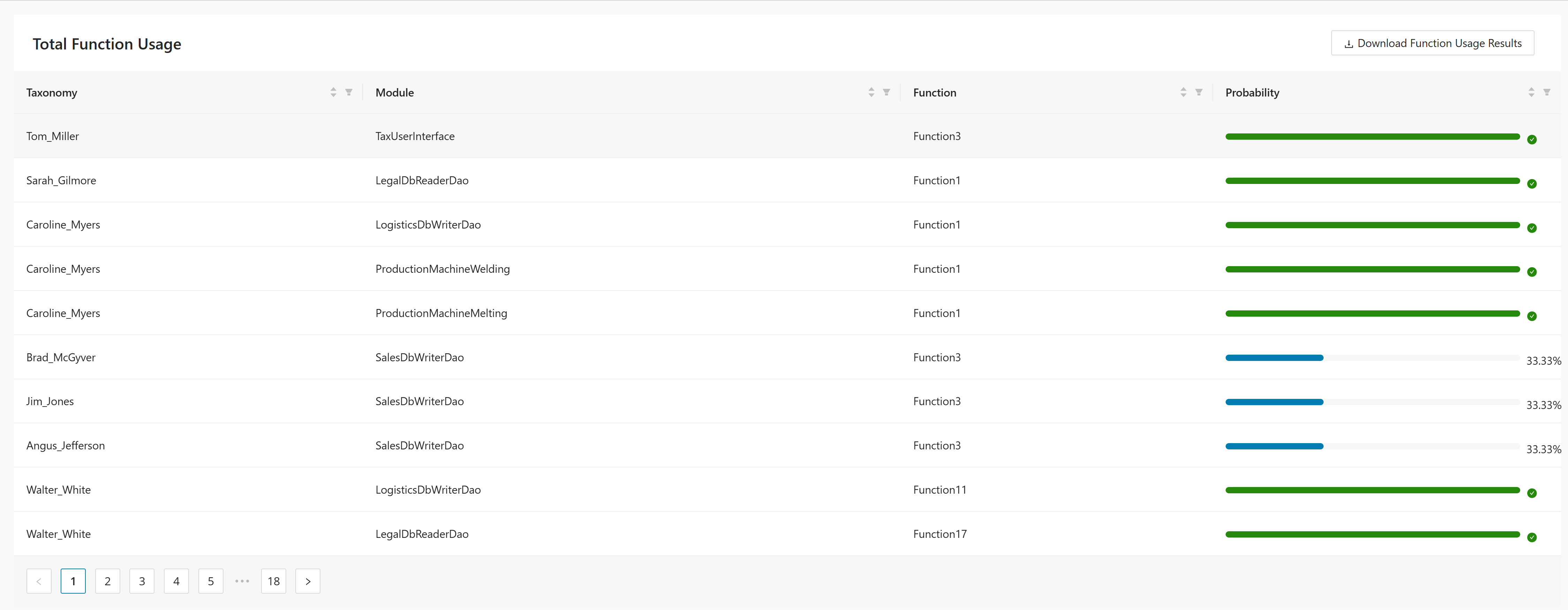
Use this page as follows:
- Review the Taxonomy, Module, Function, and Probability columns.
- Use the pagination controls to move through the result set.
- Click Download Function Usage Results to export the current report.
Social graph
The Social Graph report visualizes relationships around a selected taxonomy and supports graph export.
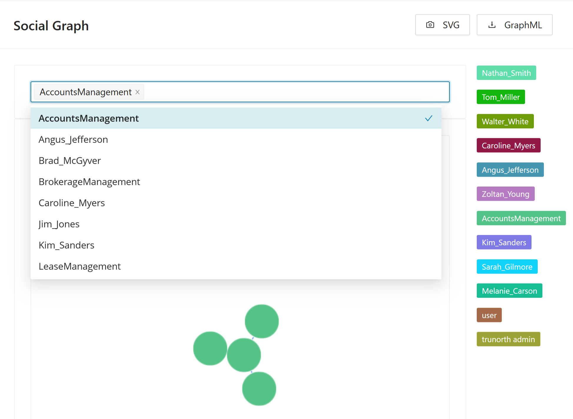
Use this page as follows:
- Select a taxonomy from Select specific taxonomy.
- Review the generated graph for the selected taxonomy.
- Click SVG or GraphML to export the current graph.
If the project does not yet contain taxonomy data, the page cannot generate the graph.
Taxonomy graph
The Taxonomy Graph report visualizes the selected taxonomy and supports SVG export.
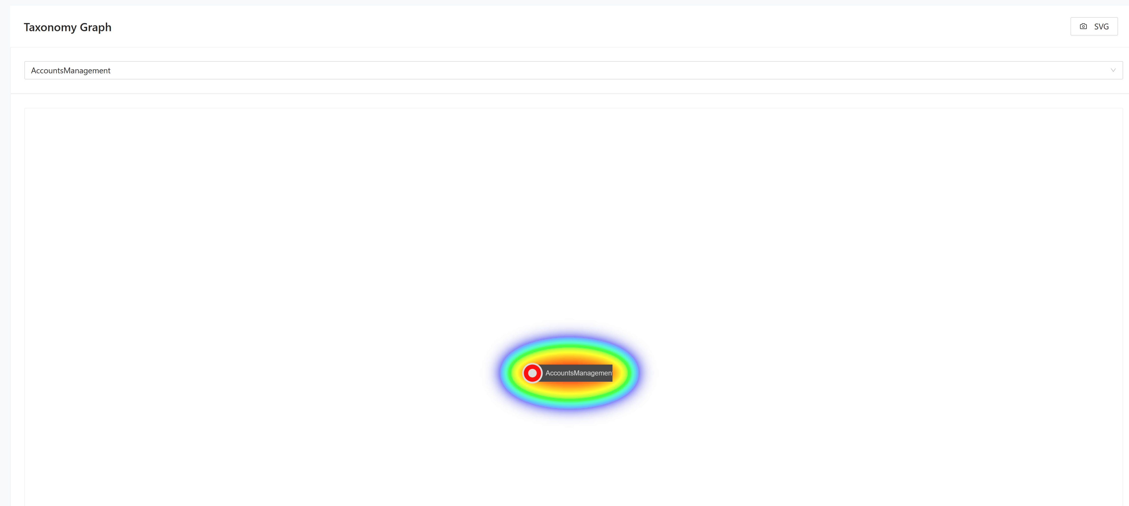
Use this page as follows:
- Select a taxonomy from the drop-down list.
- Review the generated business process graph for the selected taxonomy.
- Click SVG to export the graph.
About Tracer
The About section in Tracer contains the conceptual pages that explain how Tracer collects runtime evidence, maps users to taxonomies, and calculates module affiliation probabilities. This page introduces the problem that Tracer solves and the high-level solution behind the feature. It explains why runtime evidence matters when static analysis alone cannot assign modules confidently to business domains. Read this section before configuring tracing data or reviewing probability outputs.
The problem statement:
It is difficult to determine which part of the codebase belongs to which taxonomy, but this knowledge is extremely useful for a successful migration from a monolithic legacy system to a modern application that is decomposed into domains and sub-domains.
Manual determination of the affiliation of a module to a taxonomy is very time consuming and error prone.
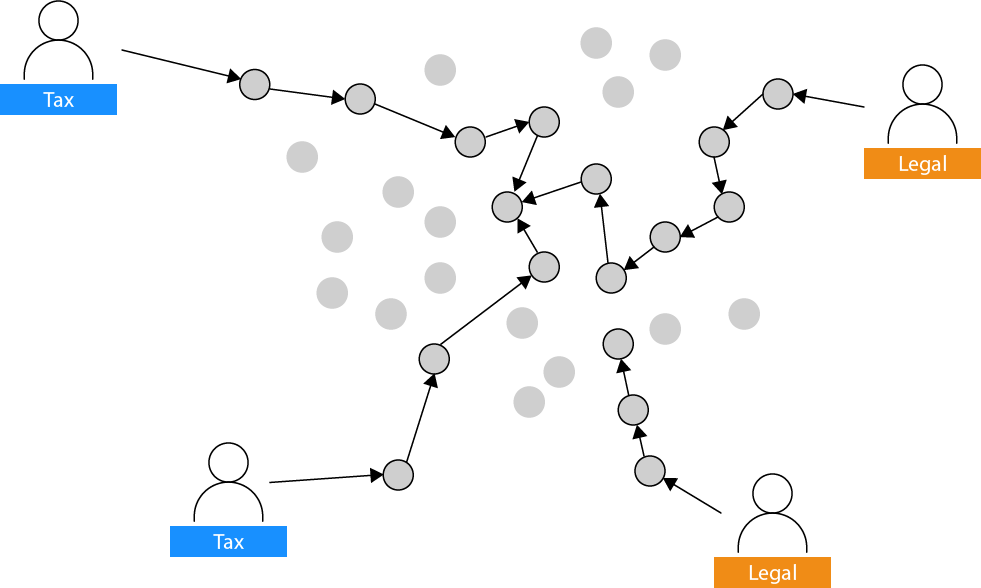
The solution approach:
Tracer follows the user through the system.
Combined with the knowledge which users is mapped to which taxonomy, Tracer can automatically determine the affiliation of a module to a taxonomy.
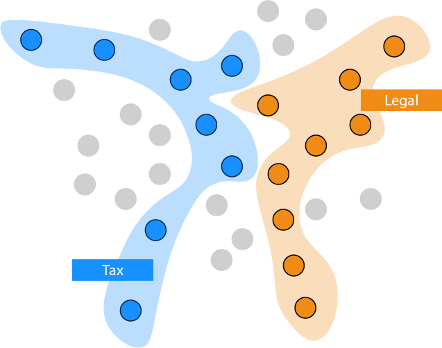
Application Overview
The Application Overview page explains the Tracer data model and the main entities that participate in the calculation flow. It shows how projects, users, taxonomies, modules, functions, and logs fit together in one analysis pipeline. Review this section when you need to understand what data Tracer expects and how the result calculation is derived.
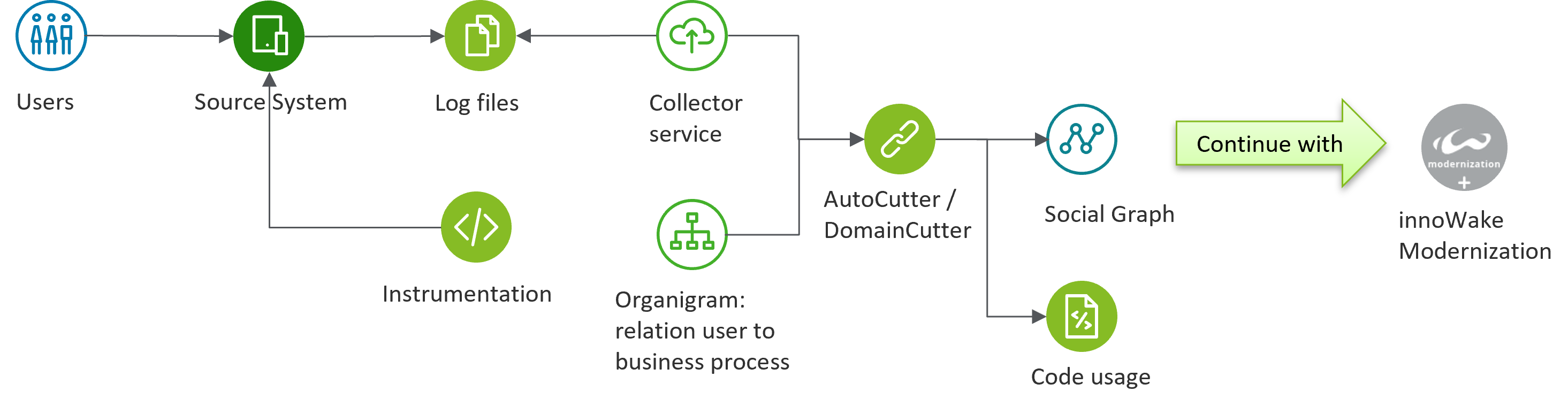
The Tracer architecture uses log files and organigrams to calculate each module's taxonomy affiliation.
| Topic | Description |
|---|---|
| Project | A Project is the top element of all other entities and contains assigned application details. New projects can be added on the project page. |
| User | Users, or more precisely actors, perform actions on a legacy application. Each user has at least one identification that can be found in the log files of the legacy application. Users can be identified automatically by the log file parser, or can be imported or manually input on the user input page. |
| Taxonomy | The knowledge about actual taxonomies does not exist within the static source code of the legacy application, therefore it must be given to the Tracer. Taxonomies can be defined manually, identified by the log file, or imported on the taxonomy input page. |
| Taxonomy Mapping | Now that we have the users and taxonomies of the application, we need to create a mapping from users to taxonomies. This mapping must be done manually, or by an import on the taxonomies-to-user mapping page. Alternatively the Tracer will automatically create new taxonomies for users or actors without mapping. |
| Mining Module | A module is a class or code file of an arbitrary programming language. Each taxonomy contains multiple modules and the modules may be shared between taxonomies. Modules can be defined manually, identified by the log, or imported on the mining module page. A static code analysis and discovery tool can easily provide the available modules within the legacy system. |
| Mining Function | A function is a method, procedure, or function of a module or class of an arbitrary programming language. Each module may contain multiple functions. Functions can be defined manually, identified by the log, or imported on the mining function rendering page. |
| Database Query | A database query is a database query of a module of an arbitrary programming language. Each module may contain multiple database queries. Database queries can be defined manually, identified by the log, or imported on the database query rendering page. |
| Result Calculation | With the help of application logs and the collector framework, Tracer can trace users through the application. To make use of the data, a calculation has to be started. This calculation identifies the modules used by each taxonomy and assigns a probability to each module. The probability indicates how likely the module is part of each taxonomy. A probability of 1.0 means that the module is certainly part of the taxonomy. A lower probability decreases the confidence that the module is part of this particular taxonomy.The result of the calculation can be found on the Taxonomy Usage report page. |
| Collector | To get the user flow from an application, the logs created by the application have to be processed. This is done in the collector component of the Tracer. The collector is responsible for parsing application logs and transforming them into an internal representation that can be used to reason about the data. The collector component already ships with supported log types: - COBOL logs - Java application logs - .NET application logs - Database query logs If you want to know how you can create the log files, visit the Data Gathering page. Once the logs are created, the collector needs to parse them accordingly. If you need to parse a custom format, visit the About Data Analysis page. |
Data Gathering
The Data Gathering page explains how Tracer follows module execution across a user flow and how it identifies unused or less-used modules. It focuses on how raw execution evidence is captured and why repeated usage matters for later probability calculations. Use this section to understand what kind of runtime activity produces useful Tracer results.
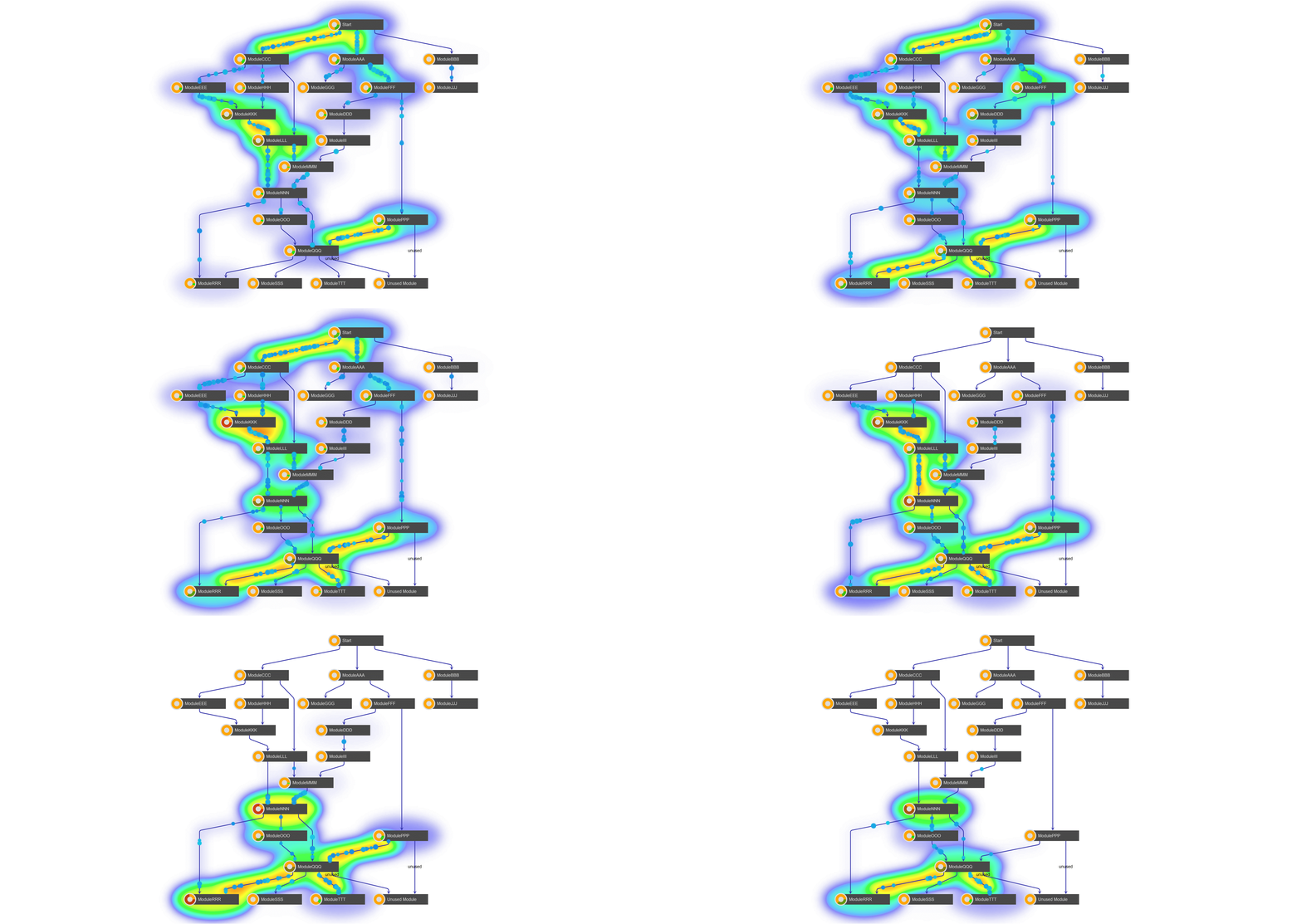
When an user starts working by starting an action in an user interface or in a batch process, the system will execute calls to modules, that will call other modules et cetera.
Not only is it possible to follow the user through the application, but the Tracer also takes into account how often a module is accessed. As a side effect, the Tracer also detects unused or less used modules.
Instrumentation
The Instrumentation page provides examples on how to instrument a legacy system so that it writes the log data required by Tracer. It is intended for teams preparing source systems to emit the runtime evidence that Tracer consumes. Use this section when you need practical guidance for COBOL, Java, .NET, or runtime-based tracing setup.
An obvious requirement for the Tracer is that we have access to a log file or another data source that contains the necessary information. The page provides examples on how to instrument the legacy application to write log files. As an alternative to the provided examples, you can also create a custom log writer and parser.
How to Instrument COBOL Applications
The script walks through all COBOL code and inserts in each call of each module a log message.
Download the instrumentation script
How to Instrument Java Applications
Run the agent together with your application. The agent will hoop into the Java VM and create the log files that are required for AutoCutter. The agent must be added as an option to the Java VM while starting the instrumented application.
Download the Tracer java agent
Download the Tracer java agent parameter file
How to Instrument .NET Applications
Run the agent together with your application. The agent will hook into the .NET application and create the log files that are required for Tracer.
Download the Tracer .net agent
How to Instrument the innoWake Runtime
Programs that are using the innoWake Runtime can use existing hooks in the runtime to write log messages.
Open Telemetry
The Open Telemetry page explains how OpenTelemetry Auto Instrumentation can be used instead of custom Tracer instrumentation. It is useful when you want to rely on a more standard observability stack while still producing trace data for Tracer analysis. Review this section if your environment already uses OpenTelemetry or you want to avoid custom logging agents.

Open Telemetry Instrumentation Overview
The Tracer architecture includes OpenTelemetry Auto Instrumentation, a widely used tool for generating, instrumenting, collecting, and exporting telemetry data, including metrics, logs, and traces.
OpenTelemetry Auto Instrumentation is available as libraries for various languages such as Python, Java, .NET, and NodeJS, and it does not require changes to the source code. The primary idea behind using OpenTelemetry Auto Instrumentation remains consistent with the approach previously described on the about tracer page, with the key difference being the method of log generation.
Instead of using custom Tracer instrumentation, OpenTelemetry Auto Instrumentation is employed. The advantage of this approach is that OpenTelemetry Auto Instrumentation is widely accepted and used by many companies.
Open Telemetry Agent Configuration
By default, OpenTelemetry Auto Instrumentation does not include user information in trace data, which is crucial for Tracer to analyze log files effectively.
To enable this, you need to configure the OpenTelemetry Agent by adding the appropriate environment variables, as demonstrated in the example configuration below. Additionally, the agent needs to know where to send telemetry data, so the Open Telemetry Collector Endpoint must be configured.
For more details on agent configuration, refer to the official OpenTelemetry documentation:
In the Tracer architecture described above, the Telemetry Service can generate output files for multiple source code apps simultaneously. This is achieved by adding the source code name to each span, which is configured using the OTEL_SERVICE_NAME environment variable, as demonstrated below.
Open Telemetry Collector Configuration
The Open Telemetry Collector provides a vendor-neutral solution for receiving, processing, and exporting telemetry data. It enhances scalability and supports a variety of open-source observability data formats, including Jaeger, Prometheus, and Fluent Bit, allowing seamless integration with both open-source and commercial backends.
In the Tracer architecture described above, the OpenTelemetry Collector functions as a telemetry message producer, using Kafka for exporting these messages. It preprocesses telemetry messages from the agent and sends them to Kafka with predefined topic names.
Below is a sample configuration for the OpenTelemetry Collector. It is important to ensure that the Kafka exporter protocol version matches the Kafka version in use, and that the encoding is set to the Jaeger JSON format.
Telemetry Service
The Telemetry Service generates input log files on a scheduled basis for Tracer by subscribing to telemetry Kafka topics produced by the Open Telemetry Collector.
Download the Tracer sample logs
About Data Analysis
The About Data Analysis page explains how to extend the collector with a custom parser for a custom log format. It is intended for cases where the shipped collectors do not match the logging format used in your legacy environment. Use it when you need to adapt Tracer to a non-standard source of runtime evidence.
How to Write a Custom Log Processor
The Tracer extracts information about the usage of the code modules of a legacy system from its log files. It calculates how often a user has accessed a module. Combined with the knowledge about the taxonomy that the user is typically working on, the Tracer can derive probabilities of the affiliation of a module to a taxonomy.
The Tracer relies on the information found in log files of legacy systems, or similar systems, like Application Performance Monitoring. While the collector application provides standard implementations for some log files, it is also possible to extend it with custom parsers for custom log files of any type.
Tracer Probability Calculation System
The Tracer Probability Calculation System is a data-driven approach to determine which bounded contexts modules and functions belong to in a microservices architecture. It analyzes actual usage patterns across different user groups to mathematically calculate the probability of module/function ownership.
Core Concepts
The probability model depends on a small set of concepts that connect users, taxonomies, and recorded usage. Understanding these terms first makes the later formulas and examples much easier to follow. Use this section as the glossary for the rest of the calculation explanation.
| Concept | Description |
|---|---|
| Traced Taxonomy | A Traced Taxonomy represents a group of users who work in a similar domain, department, or business area. These taxonomies serve as candidate bounded contexts for your future microservices architecture. Examples: - Sales Team - Finance Department - Customer Support - Inventory Management Team |
| User Usage Tracking | The system maintains detailed records of module and function executions: - UserModuleUsage: Tracks which users executed which modules, with execution counts - UserFunctionUsage: Tracks which users executed which functions, with execution counts Each user is associated with a specific Traced Taxonomy, allowing the system to aggregate usage patterns by business domain. |
| Probability | A decimal value between 0.0 and 1.0 representing the strength of association between a module/function and a traced taxonomy: - 0.0: No usage by this taxonomy - 0.5: Moderate usage (50% of total) - 1.0: Exclusive usage by this taxonomy When displayed, probabilities are converted to percentages (e.g., 0.80 → 80.00%). |
Calculation Algorithm
This section explains how Tracer converts recorded usage into probabilities that can support bounded context decisions. The formulas are simple, but the interpretation matters because they summarize behavior across multiple users and taxonomies. Review these calculations before using the results as architectural evidence.
Module Probability Calculation
Formula:
Example Calculation:
Module: CustomerOrder
| Traced Taxonomy | Usage Count | Calculation | Probability | Percentage |
|---|---|---|---|---|
| Sales Team | 80 | 80/100 | 0.80 | 80.00% |
| Finance Team | 15 | 15/100 | 0.15 | 15.00% |
| Support Team | 5 | 5/100 | 0.05 | 5.00% |
| TOTAL | 100 |
Conclusion: CustomerOrder module has the highest probability (80%) for the Sales bounded context.
Function Probability Calculation
The same logic applies but at the function level. Additionally, it weights the calculation by both:
- Number of users in the taxonomy
- Total count of function executions per user
Formula: probability = (usageCount * numberOfUsersInTaxonomy) / totalUsage
This ensures that taxonomies with more active users get appropriate weight in the calculation.
Implementation Details
The implementation details describe how raw probability values are presented to users in the product and related outputs. This helps you interpret what you see in the UI and exported reports without having to work directly with decimal values. Use this section when you want to align the mathematical model with the displayed results.
Display Formatting
Probabilities are converted to percentages for user display:
Example: 0.8534 → 85.34%
Use Cases
The use cases show how the probability system supports practical decomposition decisions instead of remaining a purely theoretical model. They illustrate how to interpret balanced versus dominant probabilities in real modernization scenarios. Use these examples to translate Tracer output into next actions for architecture work.
1. Bounded Context Suggestions
Scenario: You want to decompose a monolithic database into microservices and need to decide which modules belong to which bounded context.
Solution: Query the most probable usage results: Each module will show its highest probability taxonomy, suggesting the best bounded context assignment.
2. Identifying Cross-Cutting Concerns
Scenario: Some modules are used across multiple domains and should be shared services.
Solution: Look for modules with similar probabilities across multiple taxonomies:
Example Result: - Logging Module: Sales 35%, Finance 33%, Support 32% → Shared Service - Customer Module: Sales 85%, Finance 10%, Support 5% → Sales Bounded Context
3. Monitoring Domain Evolution
Scenario: Track how module usage patterns change over time.
Solution: Recalculate probabilities periodically and compare trends:
Conclusion
The Tracer Probability Calculation System provides a data-driven, mathematical approach to bounded context identification. By analyzing actual usage patterns across user groups, it removes guesswork from microservices decomposition and provides quantifiable evidence for architectural decisions.
Key Takeaway: Let your users' behavior guide your architecture decisions, not just theoretical domain models.
Use cases
This page groups common Decompose workflows into practical use cases that you can follow during project delivery. Each section describes a typical goal, the main prerequisites, and the steps to complete the task in the product. Use these scenarios as quick-start playbooks when you need to map a business question to a concrete Decompose workflow.
Imports use cases
These import scenarios focus on getting the core project data into Decompose so later analysis features have the right inputs. They cover both direct database extraction and handoff from Mining-based workflows. Use these examples when you need a practical path for loading a new project.
I want to get database schema information from the legacy database of the customer
Prerequisites:
- Clarify with the customer whether a DDL export tool is available, or whether DB-Crawler will be used.
Step 1: Export the database schema from the legacy system.
- Option 1: Export the DDL with the customer-provided tooling and collect the SQL file.
- Option 2: Run DB-Crawler against the legacy database and collect the JSON output.
Step 2: In Decompose, open Imports > Schema Upload.
Step 3: Upload the SQL or JSON file and start the import.
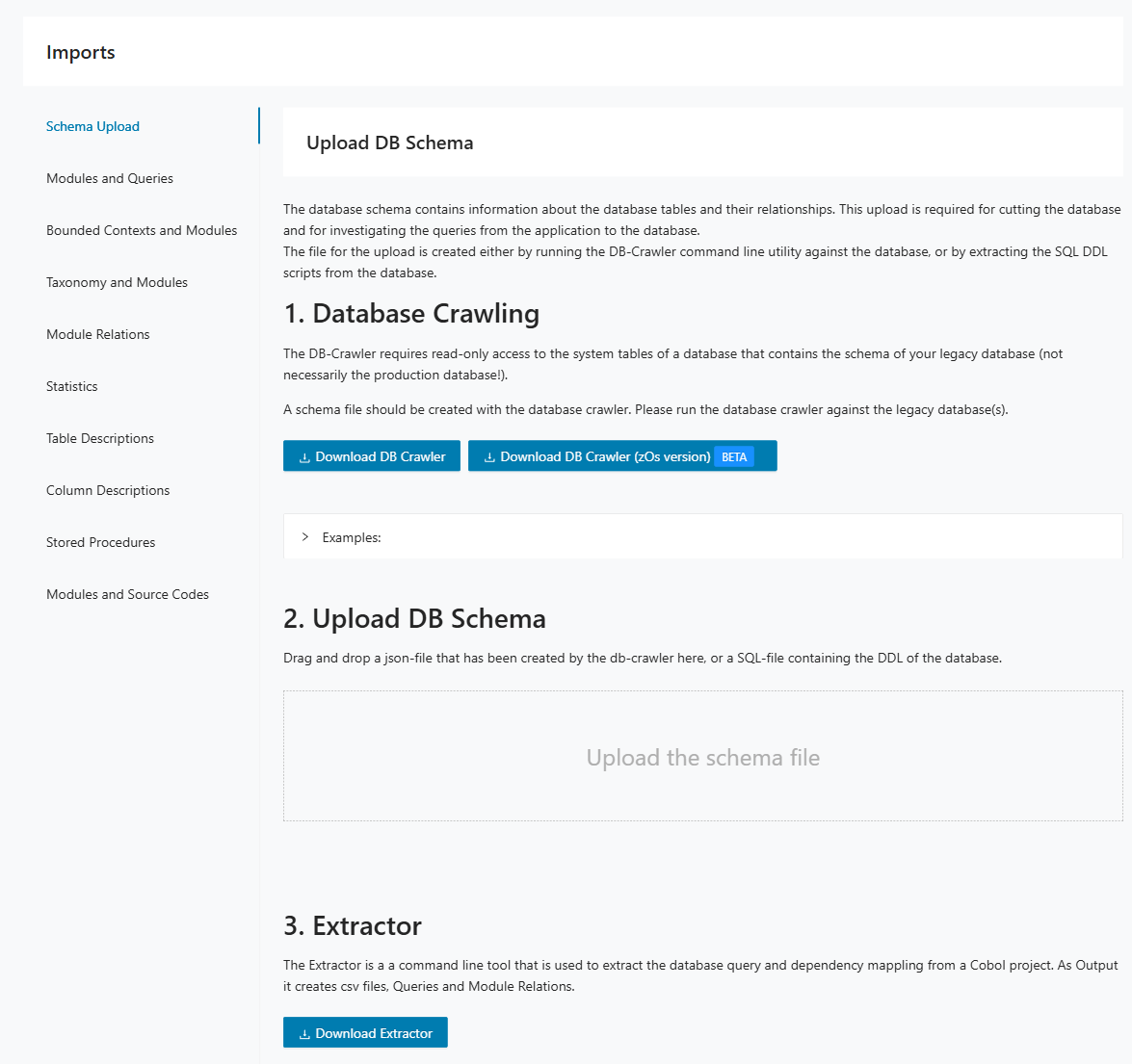
Step 4: Verify that expected schemas, tables, and views are available for downstream analysis.
Step 5: Continue with module and query imports so Decompose can link code and database objects.
I want to connect to Mining data
Prerequisites:
- In Mining, a Discovery run has been completed.
- Optional: In Mining, taxonomies have already been assigned to modules.
Step 1: Install the DB-Cutter Mining plugin in Mining.
Step 2: Export CSV files from Mining: Modules and Queries, Module Relations, and optionally Taxonomies and Modules plus Source Code.
Step 3: Clean and normalize the CSV files before import. Remove irrelevant rows, align naming conventions, and keep only project-relevant content.
Step 4: In Decompose, open Imports > Modules and Queries and upload the CSV file.
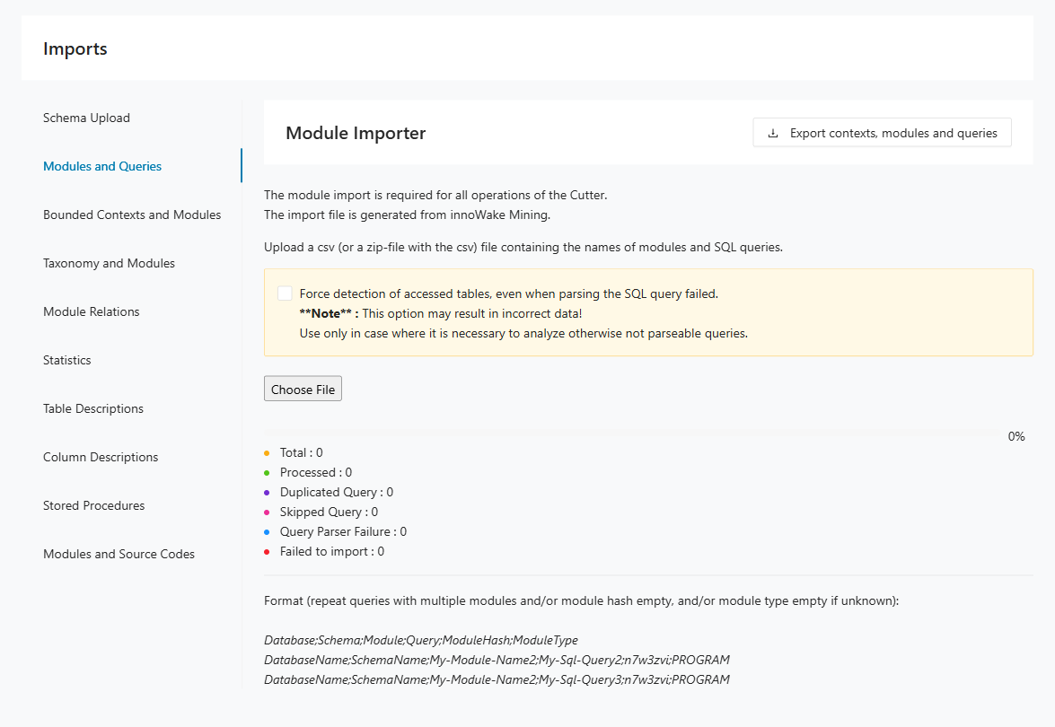
Step 5: Optional: open Imports > Taxonomy and Modules and upload taxonomy mappings.
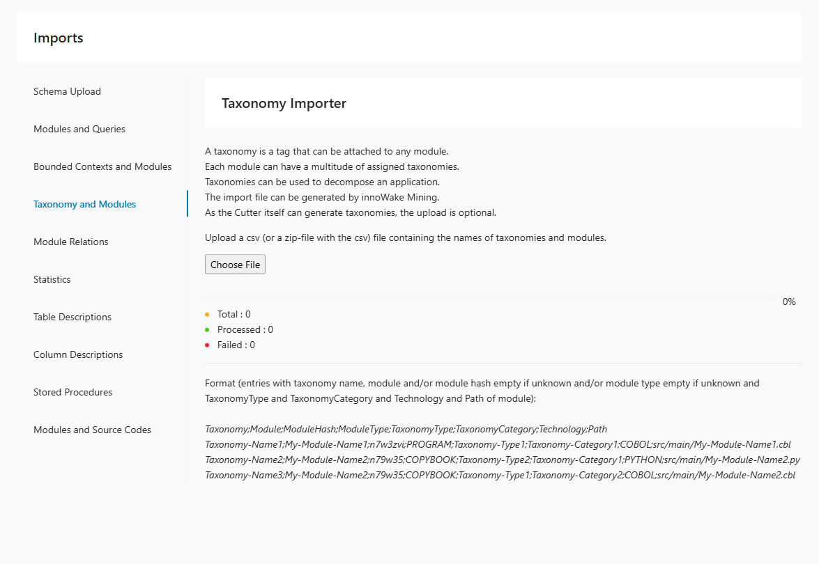
Step 6: Open Imports > Module Relations and upload module relation data.
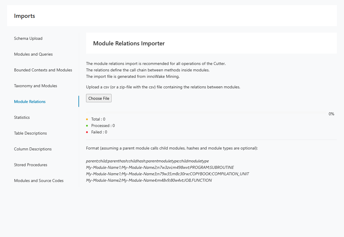
Step 7: Optional: open Imports > Modules and Source Codes and upload source code mapping data.
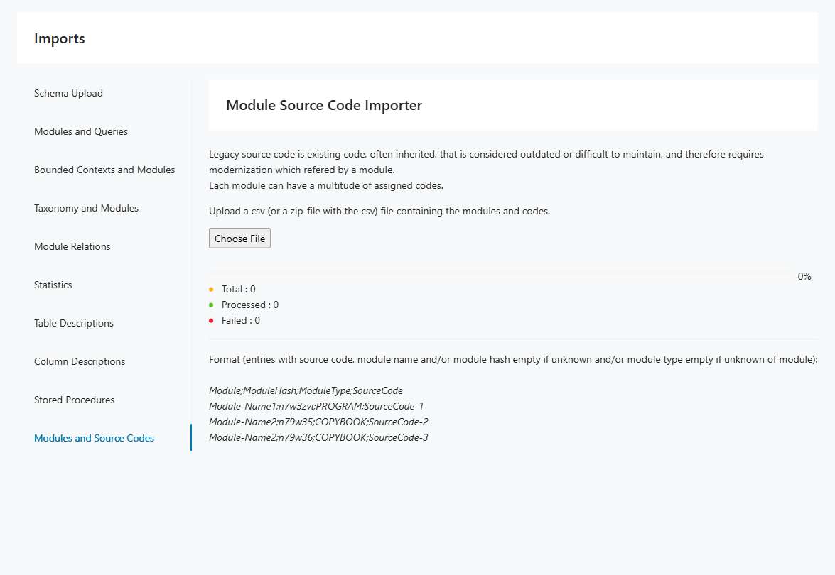
Step 8: Review import counters and error messages before moving to Insights and Decomposition.
Tracer use cases
These Tracer scenarios show how runtime evidence can support taxonomy discovery, behavior-driven decomposition, and dead-code analysis. They are useful when static analysis alone does not provide enough confidence about system usage. Use them to plan tracing activities around concrete modernization questions.
I want to identify a taxonomy in a code base
Prerequisites:
- The code base is supported by OpenTelemetry (Language APIs & SDKs | OpenTelemetry).
- We have access to the running system, ideally in a TEST environment.
Step 1: Instrument the code base with OpenTelemetry outside Decompose.
Step 2: Run the application and execute the relevant business case.
Step 3: Collect the generated log file or files.
Step 4: In Decompose, open Tracer > Upload Logfile and import the log file(s).
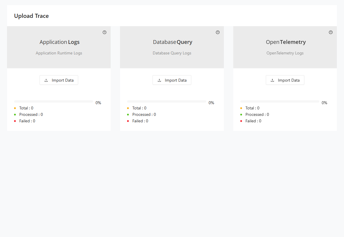
Step 5: Open Tracer > Reports > Taxonomy Usage and export the report.
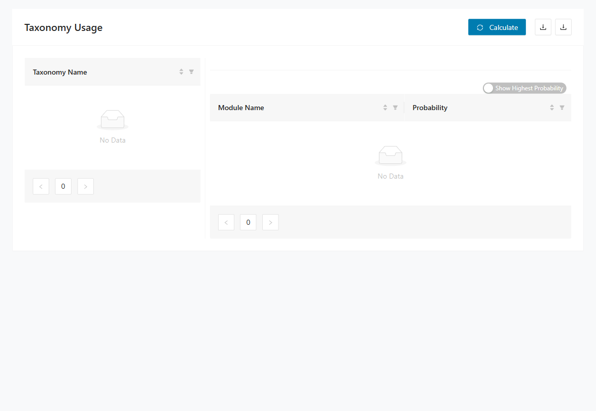
Step 6: Use the report to validate taxonomy assignments and refine decomposition boundaries.
I want to decompose a code base by user behavior
Prerequisites:
- The code base is supported by OpenTelemetry (Language APIs & SDKs | OpenTelemetry).
- We have access to the running system in a PROD environment.
Step 1: Instrument the code base with OpenTelemetry outside Decompose.
Step 2: Run the application for a representative period.
Step 3: Let users work as usual to capture realistic behavior.
Step 4: In Decompose, open Tracer > Upload Logfile and import the collected log file(s).
Step 5: Open Tracer > Reports > Taxonomy Usage and export the report for behavior-driven decomposition planning.
I want to identify dead code in a code base
Prerequisites:
- The code base is supported by OpenTelemetry (Language APIs & SDKs | OpenTelemetry).
- We have access to the running system in a PROD environment.
- A static code analysis has been performed (for example, with Mining).
Step 1: Instrument the code base with OpenTelemetry outside Decompose.
Step 2: Run the application and collect logs during normal usage.
Step 3: In Decompose, open Tracer > Upload Logfile and import the log file(s).
Step 4: Open Tracer > Reports > Module Usage and export the report.
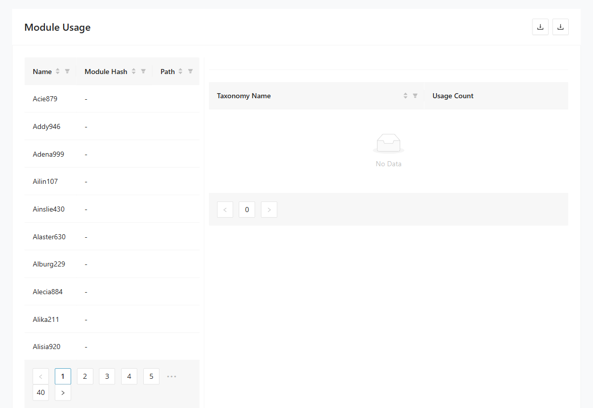
Step 5: Compare runtime activity with static analysis results to identify dead-code candidates.
Insights use cases
These Insights scenarios focus on understanding how modules, tables, and views relate to each other in the imported system. They help you answer targeted questions about table access and query behavior before making decomposition decisions. Use them when you need evidence from the analysis views rather than from tracer data or DB cutting.
I want to identify the modules that query a table
Prerequisites:
- Modules and queries have been imported.
Step 1: Open Insights > Query Paths.
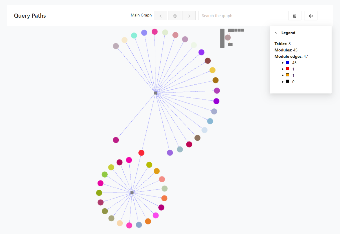
Step 2: Search the graph for a table name or module name.
Step 3: Select the table node.
Step 4: Review connected modules to identify who reads or writes the table.
I want to identify the modules that query a table in detail
Prerequisites:
- Modules and queries have been imported.
Step 1: Open Insights > Access Pattern Analysis.
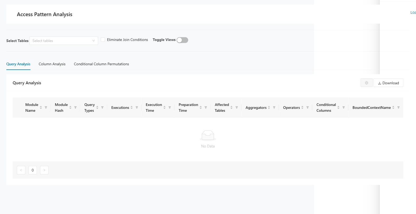
Step 2: Search for the target table.
Step 3: Review query characteristics and module-level access details.
Step 4: Open Insights > Reports > Module Table Access and export the report.
I want to identify tables that are queried by a view
Prerequisites:
- Modules and queries have been imported.
Step 1: Open Insights > Reports > Views and Tables.
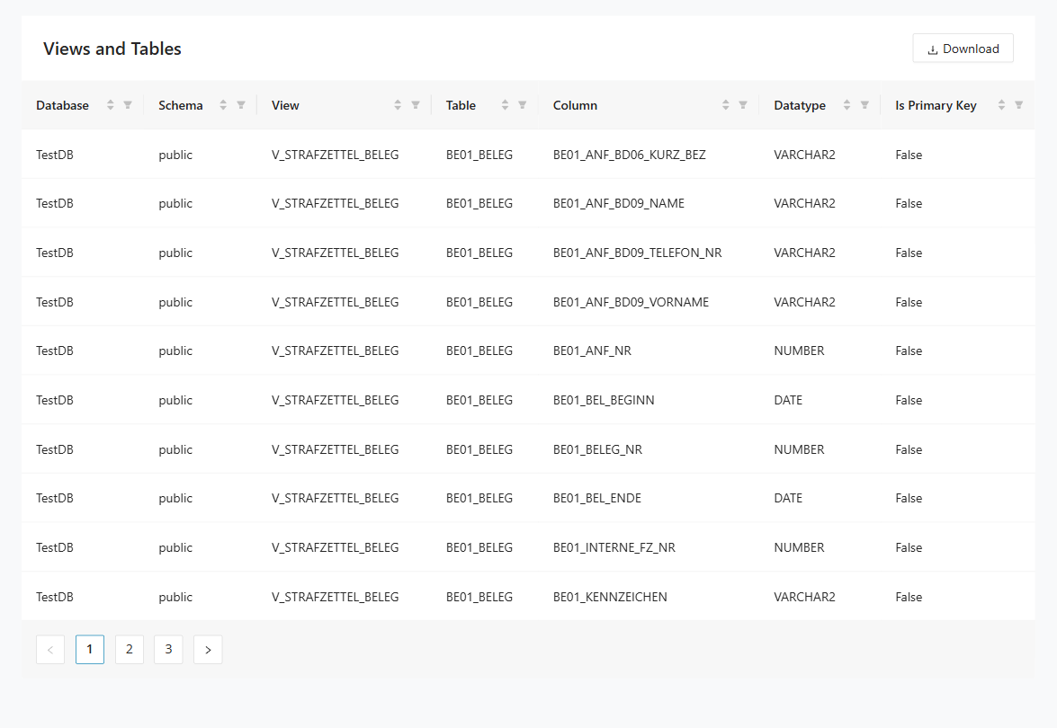
Step 2: Filter by view name to list related tables and columns.
Step 3: Export the Views and Tables report.
Decomposition use cases
These Decomposition scenarios help you turn imported module data into taxonomies and bounded context candidates. They are intended for teams actively shaping context boundaries and reducing cross-domain dependencies. Use them when you are refining how the application should be split into coherent domains.
I want to tag all modules in a call chain that accesses a table
Prerequisites:
- Modules and queries have been imported.
- Module relations have been imported.
Step 1: Open Decomposition > Reachability Analysis.
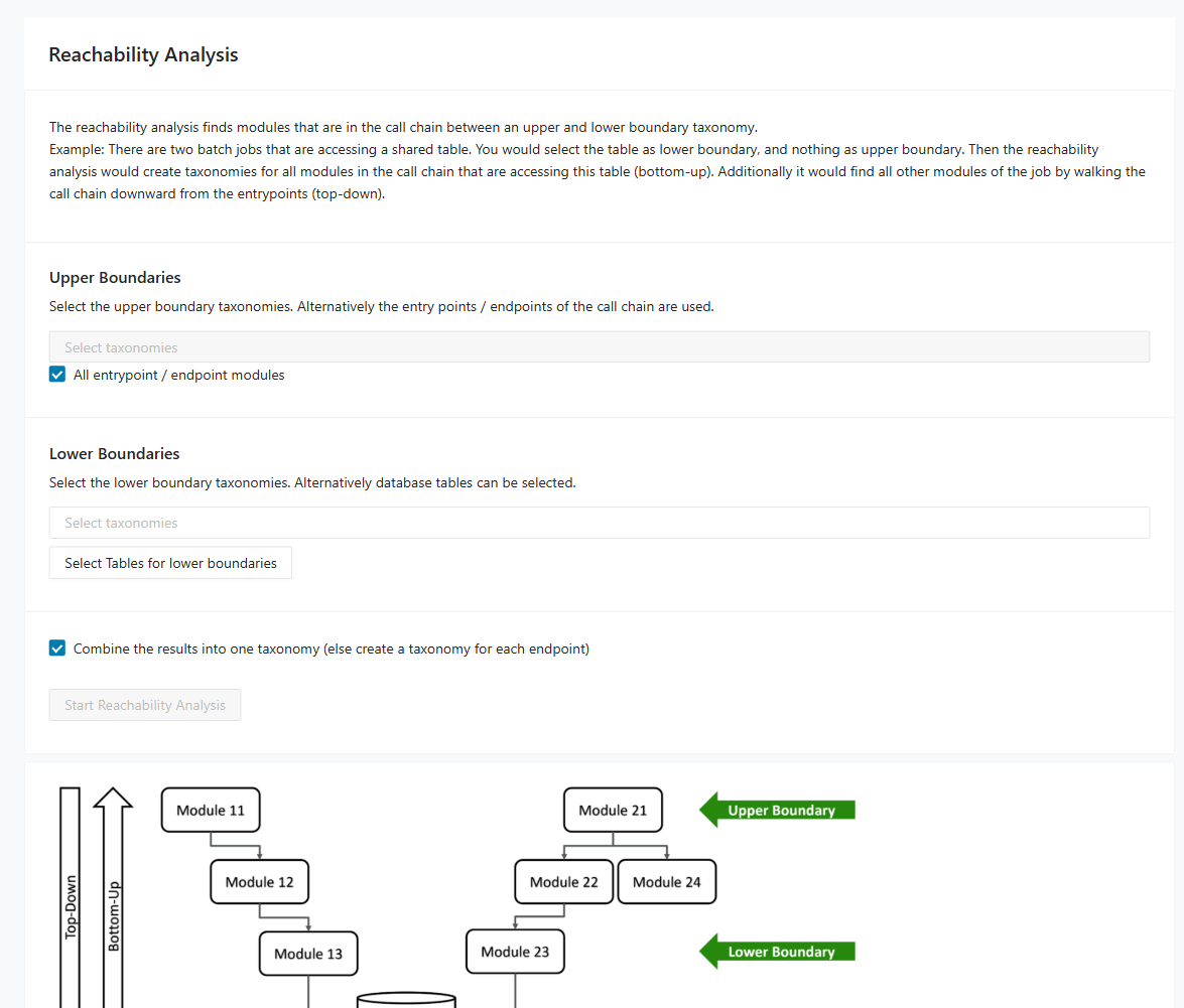
Step 2: Select the relevant upper and lower boundaries.
Step 3: Keep Combine the results enabled to create one taxonomy over all matching call chains.
Step 4: Disable Combine the results to create one taxonomy per endpoint.
Step 5: Run the analysis and review created taxonomies prefixed with RA.
I want to minimize code dependencies between taxonomies
Prerequisites:
- Modules and queries have been imported.
- Module relations have been imported.
- Optional: Mark taxonomies as Bounded Context Candidate in the Taxonomy Editor.
Step 1: Open Decomposition > Taxonomy Graph.
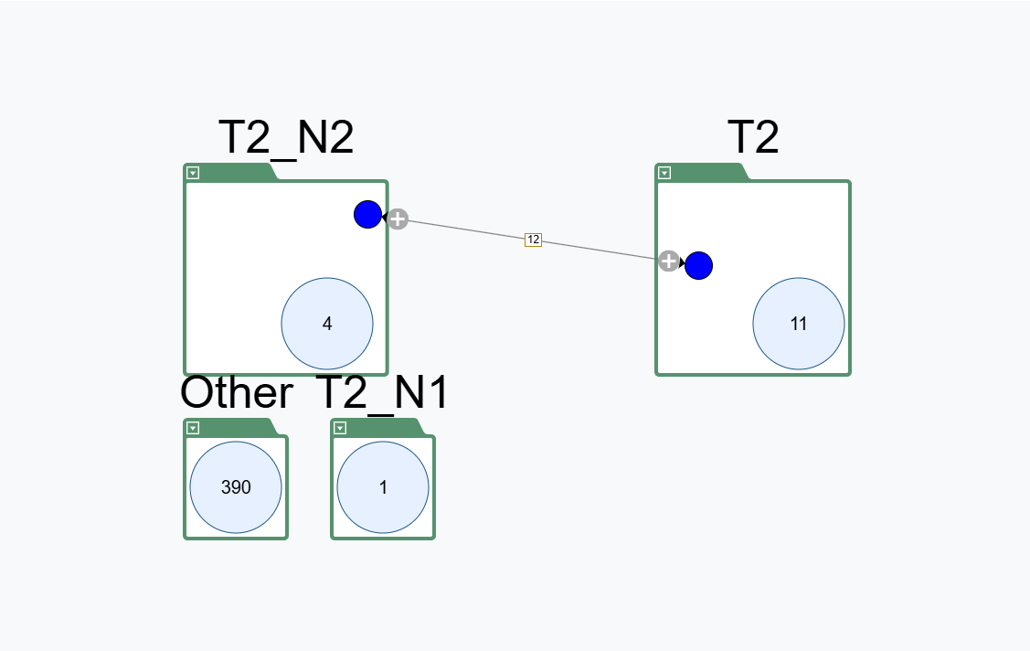
Step 2: Add the relevant taxonomies to the graph.
Step 3: Right-click a taxonomy and add intersection taxonomies where needed.
Step 4: Move modules between taxonomies and intersections to reduce cross-taxonomy dependencies.
I want to use Mining Taxonomies as Bounded Contexts for DB Cutting
Prerequisites:
- Modules and queries have been imported.
- Optional: Mark taxonomies as Bounded Context Candidate in the Taxonomy Editor.
Step 1: Open Decomposition > Bounded Context Editor.
Step 2: Go to the Taxonomy to Context tab.
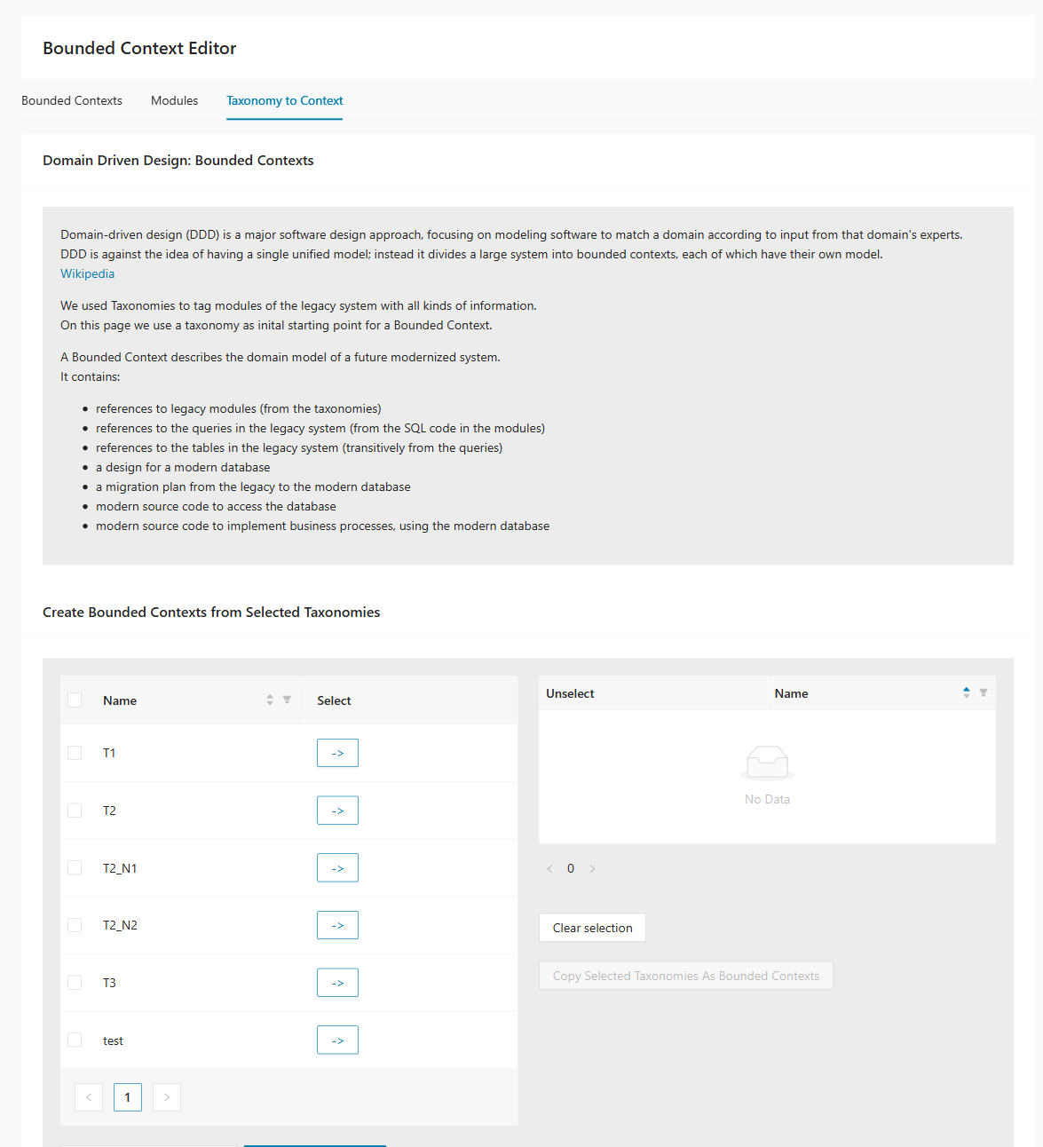
Step 3: Select the taxonomies that should become bounded contexts.
Step 4: Click Copy Selected so one bounded context is created for each selected taxonomy.
DB Cutting use cases
These DB Cutting scenarios focus on discussing and deciding how legacy tables and columns should move into target bounded contexts. They are useful in workshops where technical and business stakeholders need to review decomposition options together. Use them when you want to move from analysis into database-level design decisions.
I want to discuss the database decomposition with the customer (high level)
Prerequisites:
- Modules and queries have been imported.
- Database schema has been imported.
- A bounded context has been defined.
Step 1: Open DB Cutting > Table Decomposer.
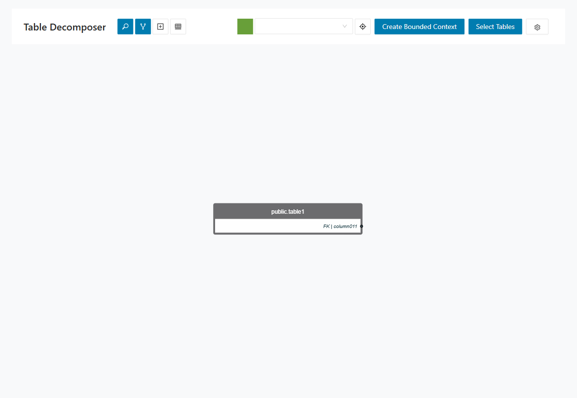
Step 2: Select the bounded context to discuss.
Step 3: Enable Show Primary Key and Show Foreign Key.
Step 4: Review the graph with the customer.
Step 5: Right-click tables to assign them to the bounded context or add related tables to the view.
I want to discuss the database decomposition with the customer (detail level)
Prerequisites:
- Modules and queries have been imported.
- Database schema has been imported.
- A bounded context has been defined.
Step 1: Open DB Cutting > Cut by Module.
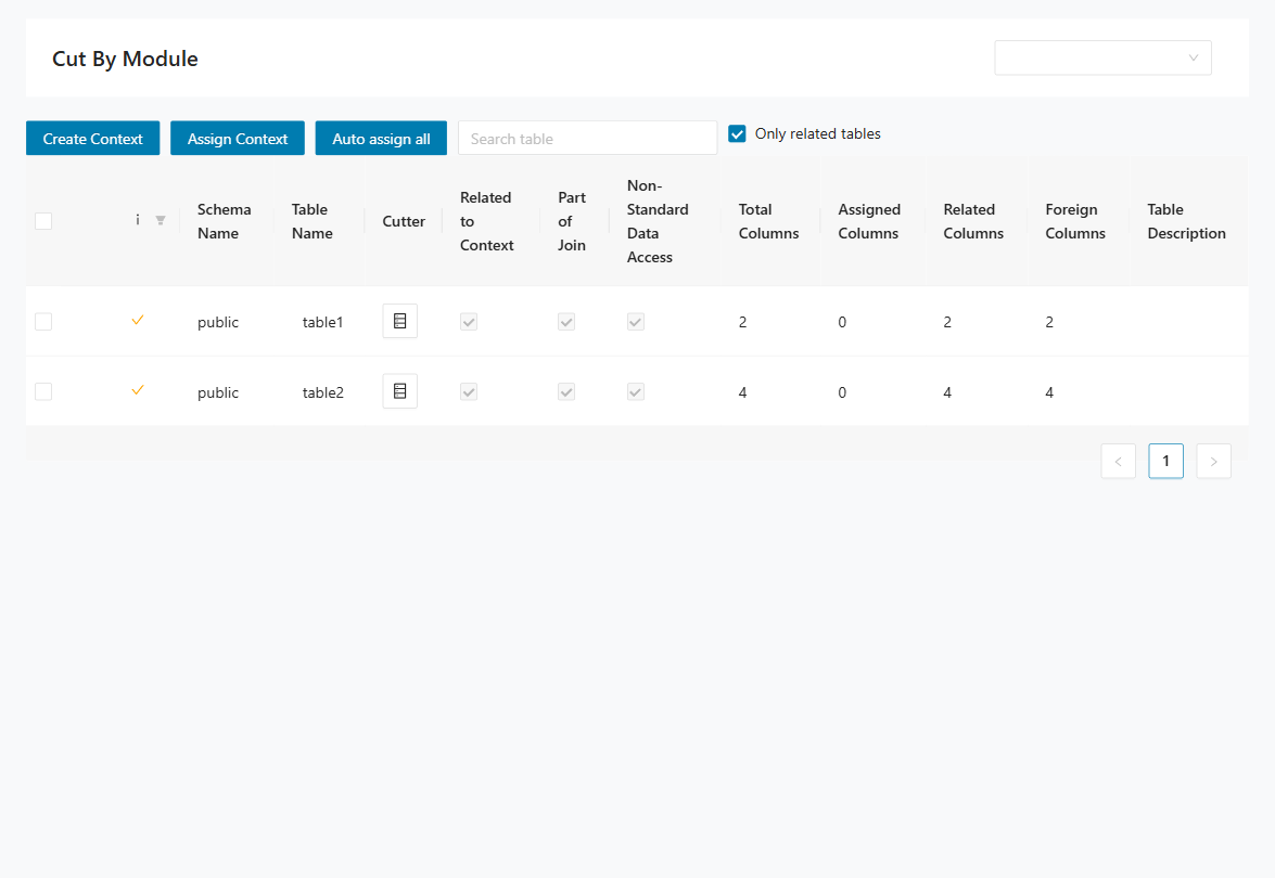
Step 2: Iterate through relevant tables and prepare a migration proposal for each column. Use this strategy guidance:
- Keep in current context: Column stays in the current bounded context.
- Move to target context: Column ownership moves to a different bounded context.
- Duplicate temporarily: Column exists in two contexts during transition.
- Expose via interface: Keep the data in one provider context and access it through an interface.
- Defer decision: Mark open points for follow-up workshops.
Step 3: Review each table and column with the customer and agree on the final strategy.
Step 4: Record customer decisions and constraints in the comment field for traceability.
Step 5: Open DB Cutting > Entities Designer to review the target schema.
Release Notes
Imprint
Germany
Deloitte innoWake GmbH
Robert-Bosch-Str. 1, D-89250 Senden
Phone: +49.7307.92190.111
Mail: amiproductsupport@deloitte.com
United States
Deloitte LLP 30 Rockefeller Plaza, New York, NY 10112
Phone: +1.800.769.0480
Mail: amiproductsupport@deloitte.com
Deloitte refers to one or more of Deloitte Touche Tohmatsu Limited, a UK private company limited by guarantee ("DTTL"), its network of member firms, and their related entities. DTTL and each of its member firms are legally separate and independent entities. DTTL (also referred to as "Deloitte Global") does not provide services to clients. In the United States, Deloitte refers to one or more of the US member firms of DTTL, their related entities that operate using the "Deloitte" name in the United States and their respective affiliates. Certain services may not be available to attest clients under the rules and regulations of public accounting. Please see http://www.deloitte.com/about to learn more about our global network of member firms. © 2026. Deloitte. All rights reserved
© 2026. Deloitte. All rights reserved.