
About this manual
This manual introduces Code Discovery & Mining, which belongs to Deloitte's Ascend Mainframe Insight and must be licensed separately. It explains the core capabilities, supported technologies, and workflows that take you from discovery into deeper analysis. Use it as the starting point for the Mining documentation set.
Introduction
The Code Discovery & Mining product provides code analytics to (re-)gain an understanding of an application.
The product offers insights into an application's scope, structure, and business value with features such as project metrics, field tracing, dependency views, business domain mapping, as well as business logic and rule extraction - all of which are stored in a sophisticated metadata repository that can be accessed from a Web application, Eclipse plugin, or a platform API.
Code Discovery & Mining supports Java and a variety of mainframe-oriented/legacy languages, including IMS, COBOL, C, Assembler, PL/1, Natural, and JCL.
Code Discovery & Mining starts with a code ingestion performed through code discovery. Once discovery is completed, users can deep dive into the application.
Getting Started
Environment setup
This chapter focuses on Code Discovery & Mining server configuration, setting up the server connection, and configuring logging. It includes detailed information about user and access management for system administrators.
Info
Code Discovery & Mining is not compatible with the IBM AIX operating system and the IBM JRE.
Postgres setup
The following section covers the setup for Postgres. It summarizes the base database tasks that Mining depends on, including cluster initialization, server startup, and initial user creation. Use the platform-specific steps below to prepare a Postgres instance before connecting the rest of the Mining components.
Windows
Perform the steps below to set up Postgres on a Windows machine.
Step 1:
Download and unpack server binaries.
-
Download the ZIP with the binaries (not the installer) from https://www.enterprisedb.com/download-postgresql-binaries.
-
Unpack the server binaries to a location of your choice (for example.
<home>/Development/postgresql). From the ZIP file, you will get a folder named pgsql ().
Step 2:
Create and initialize a new database cluster.
-
Choose a folder for creating a new database "cluster" (
). This will contain all the databases managed by a server instance along with its configuration. -
Initialize the data cluster. From the command prompt, run the code below. Note that
and should contain the absolute paths.
<pgsql>\bin\initdb --no-locale –-encoding=UTF8 <pgdata> -
After initialization, you will find the following configuration files in
. (No change is required in these files when starting the server locally.) -
postgresql.confContains basic server settings like the TCP port (5432 by default), load, and memory limits. -
pg_hba.confDefines access restrictions. By default, administrative access is allowed without authentication from localhost only.
-
Step 3:
Start the database server.
-
From a command prompt, run:
<pgsql>\bin\postgres -D <pgdata>
The server log will be printed to the terminal in real-time.Alternatively, the server can be started using a batch file as:
<pgsql>\bin\postgres.exe -D <pgdata>
Step 4:
Create an application user and a database.
-
With the server up and running, from a command prompt, run:
<pgsql>/bin/psql postgres
The server admin prompt shown below will be displayed:
postgres=+ -
From this command prompt,
-
Create a role "mining" as below:
CREATE ROLE mining WITH LOGIN; -
Then create the database "mining" with the role created above:
CREATE DATABASE mining WITH OWNER = mining;
-
Linux
Set up using Docker PostgreSQL image
Step 1:
Pull the latest or version 15 and above Postgres image using the command:
Step 2:
Create a Postgres container, copy the backup into it, and start the container as described below:
Step 3:
Delete and recreate the database and role:
Step 4:
Restore the backup using the following command:
Prerequisites (if Postgres image is not used)
Follow the steps below to manually install Postgres on a Linux machine:
Step 1:
Log in as a root user.
Step 2:
Install Postgres.
-
Install the repository RPM:
dnf install -y https://download.postgresql.org/pub/repos/yum/reporpms/EL-8-x86_64/pgdg-redhat -
Disable the built-in PostgreSQL module:
dnf -qy module disable postgresql -
Install PostgreSQL:
dnf install -y postgresql15-server
Step 3:
A pgsql-15 folder is visible in the "usr" directory.
Step 4:
Create a directory "postgresql" and a data directory "data15" within postgresql and assign the necessary permissions.
Step 5:
Copy the pgsql-15 folder and paste it into the postgresql directory:
cp -r /usr/pgsql-15 /usr/postgresql/pgsql-15
Step 6:
Log in as Postgres user, set the library path, and initialize the database cluster/directory:
Step 7:
After initialization, you will find the following configuration files in data15:
-
postgresql.conf -
pg_hba.conf
Step 8:
Open postgresql.conf, uncomment the following lines and add the IP address of the host machine against listen_addresses:
Step 9:
Open pg_hba.conf and add another IP address of the host machine under the section "IPv4 local connections":
Set up Postgres via Groovy script
Perform the following steps to set up Postgres via a Groovy Script.
Step 1:
Create a directory "postgres" inside the jobWorkspace and modify the permissions (chmod -R 777) of that directory.
Step 2:
Create a container with username and password, mount the volume from "<jobWorkspace>/postgres" to "/var/lib/postgresql/data15", and start the container with port 5432 and image postgres.
Step 3:
Copy the data directory (data15) from the host system and paste it into the container.
Step 4:
Start the Postgres container.
Step 5:
Verify that Postgres is running.
Step 6:
Create the application user and database as follows.
Step 7:
Add the JDBC URL in the command to start the API server.
AWS EC2 Instance
Add the following commands to the Postgres launch template in the User Data section:
Code Discovery & Mining API server configuration
This section gives an overview of the fundamentals of Mining API server configuration. It explains the default packaging model, the main startup options, and where to place customer-specific overrides. Use it to understand which settings must be supplied externally and which ones can remain at their defaults.
Configuration
The Mining API Server is delivered as a self-contained JAR file with a built-in default configuration. It is usually configured to customer specifications during the initial setup by the Deloitte project team.
Configuration
On Linux hosts, the fontconfig package must be installed as a requirement for the Excel file generation during Discovery.
Starting the Mining API server
The Mining API Server JAR only requires the Java JRE to run, and can be executed via command line interface (CLI) with the following command:
The server configuration can be adjusted by appending command-line options, for example, for application and log configuration.
Application configuration
The application's configuration can be adjusted by providing a customized YML file via the jar command line parameter --spring.config.additional-location:
Configuration options range from server details, database connection, and spring profile parameters to Job API (see Mining Job API) and Keycloak settings.
Configuration
The default YML configuration can be extracted from the server JAR file at mining-api-server-dist-<version>.jar\BOOT-INF\classes\application-default.yml and used as a template.
To simplify updating your Mining version, it is recommended to remove everything from the default YML, except for the configuration values that you need to customize.
For example, to configure the database URL and credentials, the following YML file content should suffice:
Task thread limit
For testing and debugging, it is possible to limit the number of concurrent tasks for the job execution.
In the application configuration YML file, adjust the block maximumLocalTaskThreads: under job-api::
Job thread limit
A job may initiate another job and wait for its completion. Therefore, the configurable number of concurrent jobs has been constrained to a minimum of 4. This helps to avoid a job causing a deadlock when another job is waiting or cannot run in parallel. To change the limit on the number of concurrent jobs, adjust the following property in the configuration YML file:
Warning
Setting the thread count below 4 will fail to start the server, and the corresponding error message: "APPLICATION FAILED TO START".
Discovery cache sizes
To optimize memory usage for Discover Code and Discover Metrics executions, the number of entries kept in memory for various tasks can be configured. To adjust cache sizes, adjust the following properties in the configuration YML file:
To restore the previous behavior, use the following setting, since caches use strong references:
Configuration
Reduce the result cache size if you are encountering OutOfMemory errors during Discovery.
Discovery upload size limit
During Discover Code operations, the project source code is uploaded in the background. The source upload has a default limit of 10,000,000,000 uncompressed bytes. The value is configurable to enable projects to upload archives that contain larger amounts of data via the discovery-source-upload-maximum-size parameter in the configuration YML file:
Call chain export options
Maximum CSV export lines
The CSV export of call chains is limited in the spring configuration to 5,000,000 lines by default. The value can be configured in the application.yaml file in the configuration section to improve call chain export performance:
Maximum export threads
It is possible to specify the maximum number of task threads for call chain computation.
The default value is 8. A value less than 1 will allow the runtime to use all available processors.
The value can be configured in the application.yaml file in the configuration section to improve call chain export performance:
Cookie consent
The Mining Web UI can be configured to prompt the user to consent to cookies before logging in.
The mining.cookieId property must be set at the time of deployment to enable or disable this feature.
Info
Cookie IDs are generated specifically for each client and are provided to the respective Deloitte project admin.
This property can be set in three ways:
Option 1:
Adjust the configuration YML file.
Option 2:
Pass the property as a start parameter in the server startup command.
Option 3:
Set the property as an environment variable.
Warning
For non-production environments, the cookie consent prompt can be disabled by assigning the value "DISABLED", for example. -mining.cookieId=DISABLED.
Authentication
The primary authentication approach is by default Keycloak authentication. However, for users opting for legacy authentication, they can activate the legacy authentication profile by appending --spring.profiles.active=legacy-auth when running the project. Pass the property as a start command in the api server startup command.
Alternatively, it can be configured in the application configuration YML file:
Set category for GenAI knowledge-service retrieval
You are allowed to specify the category/index to be used for querying the knowledge service by setting its value to the mining.genAI.annotationKnowledgeCategory property when running the project. This property is used for querying the OpenSearch database in the backend. The default value is VARIABLE_DESCRIPTION. This property can be passed along when starting the API server with the following command:
Alternatively, it can be configured in the application configuration YML file:
Introduced LLM response
The response format (for example, TEXT, JSON) of the configured model can now be specified via the responseFormat parameter inside the application.yaml. The default response format for Annotation Description generation is now JSON.
Warning
Make sure that the plugin specified in your application.yaml file supports JSON response format
Important: If the specified plugin does not support the JSON response format, make sure to change the responseFormat to “TEXT” in the application.yaml file.
For example, check Azure AI for endpoints hosted on Azure Cloud.
The following models (and newer) should support JSON mode:
-
gpt-35-turbo(1106)
-
gpt-35-turbo(0125)
-
gpt-4(1106-Preview)
-
gpt-4(0125-Preview)
Keycloak configuration
When the Mining API Server is to be used in conjunction with Keycloak, the authorized-access spring profile needs to be used. Otherwise, the server will fall back on the integrated default authentication without Keycloak. The application YML file should therefore contain the following content:
The HTML Display name and the Redirect URIs in the Keycloak Realm Client need to be adjusted to point to the Mining API server. This can be done in your Realm's client configuration via the Keycloak Admin UI.
The following example shows the required configuration for the HTML display name, backend, and web clients, assuming that the Mining API server is deployed to http://127.0.0.1:8080.
General configuration

Backend client configuration

Web client configuration

Info
Note that the URI http://127.0.0.1:4200 is also listed in the setting above. Port 4200 is the preconfigured default port for the Mining UI.
To support the Mining access matrix (see Access Matrix), a client-specific role mapping needs to be configured. Keycloak supports the integration of various identity providers and user federation systems. Therefore, your Mining setup can be interconnected with your Single-Sign-On (SSO) or Active Directory (AD) system.
For detailed information about individual options and Keycloak configurations, please refer to the official Keycloak documentation:
Keycloak version 22 upgrade
Building a Docker image
Step 1:
Log in to the Docker registry
Step 2:
Build the Docker image with the upgraded Keycloak jar (with the help of a Docker File) and tag it with the build version
Step 3:
Push the newly built image to the Docker registry
Keycloak URL
The /auth from the keycloak URL is removed and the new URL is changed to http://
Keycloak directory path
The path of the Keycloak directory to create/assign roles and users via the Keycloak Admin CLI has been changed to /opt/keycloak/bin/kcadm.sh
Connecting to an AWS Aurora Postgres database
You can use AWS Aurora as the "postgres" database. When authenticating with username/password, you can use the standard PostgreSQL driver, and no special configuration is needed. However, when you want to use AWS IAM authentication to access the database, you must use a special JDBC driver provided by AWS and a special configuration.
The documentation on the JDBC driver can be found here:
Note that setting the "classpath" argument on the command line does not have the desired effect for spring-boot jars. To load the JDBC driver, you must use the "loader.path" system property like so:
Info
You must put the -Dloader.path argument before the class argument (org.springframework.boot.loader.PropertiesLauncher), otherwise it doesn't work.
When the driver is loaded properly, you can use this configuration to set up IAM authentication:
Log configuration
Logging can be configured by providing a customized log4j2.xml file via the java system property -Dlogging.config:
Configuration
The default log configuration can be extracted from the server JAR file at mining-api-server-dist-<version>.jar\BOOT-INF\classes\log4j2.xml and used as a template.
Info
The existence of a log file depends on the configured log level in the log4j2.xml file. For example, if the log level is set to OFF or ERROR, no log file is created when only INFO events are triggered.
After a job has been executed from Eclipse (for example, mining > Analysis > Calculate Control Flow), the corresponding server log can be retrieved from the Logs column in Job View:

Clicking the Logs link will trigger a Windows Explorer prompt to save the log file to your desired location.
Temporary log directory
When executing Discovery jobs (Discover Code, Discover Metrics, etc.), the log output from these jobs is recorded in a temporary file, which is then automatically downloaded to the Eclipse workspace after the job finishes.
The location of the temporary folder can be reconfigured with the following adjustments:
In the application configuration YML file, add a child block log: under job-api::
A matching change must be applied to the log configuration. In the log configuration XML file, search for the appender with name="jobAppender-${ctx:job-id:-unknown}" and modify it as follows:
Mining Extensions
Mining extensions are Java classes that implement a certain interface and register some additional functionality for the Mining product. They are provided as .jar files by the Mining development team.
Extensions are registered automatically at runtime if they are put on the classpath of the Mining API server.
The following example outlines how to integrate the Decompose export extension.
The API server start command needs to be adjusted to include the library:
Additional launch parameters and escaping might apply, especially in the case of remote or automated deployments.
Mining API server connection
To work with most Mining functions, your local project must be connected to the Mining server. This can be done with or without Keycloak.
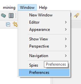
To connect to the server, navigate to Window > Preferences > mining and perform the steps for Option A: Connect with Keycloak or Option B: Connect without Keycloak, as the case may be:
Option A: Connect with Keycloak
Step 1:
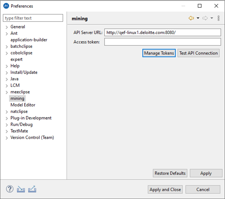
In the project or workspace Preferences, enter the correct API server URL and select Manage Tokens on the mining tab.
Step 2:
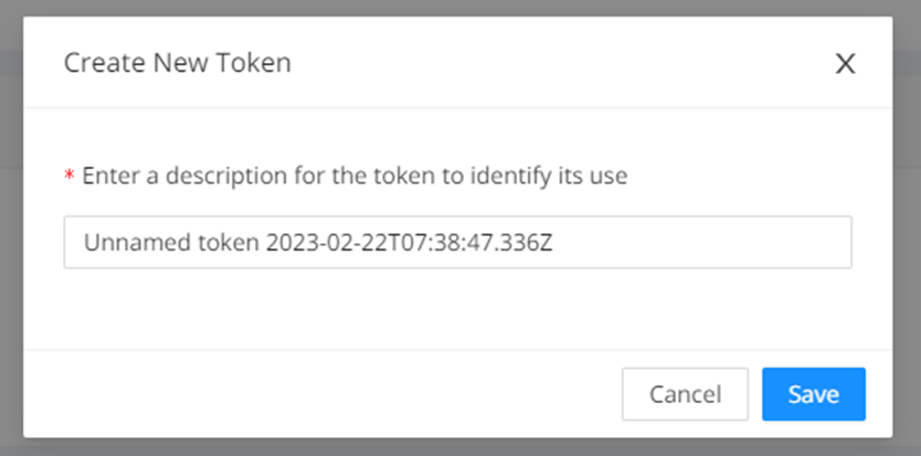
After selecting Manage Tokens , a browser opens automatically. Log on to that browser, and then click the + New Token . Enter a description (optional) in the Create New Token window. Then click Save .
Within a couple of seconds, the “Token Created” window appears with the access token. Copy the access token and close the window.
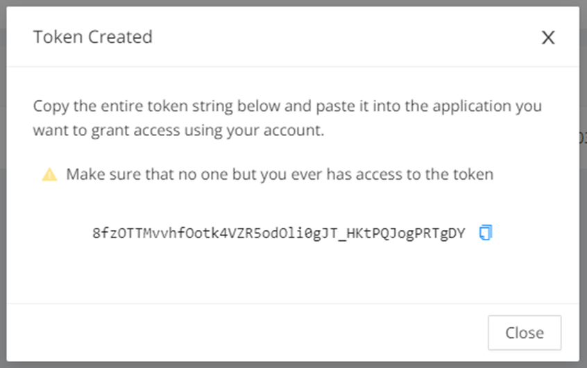
Step 3: Paste the access token in the Preferences window (see Step 1 above), click Apply , and then click the TEST API Connection . A “Server connection successful” message will be displayed along with information on the connected user, the response time, and the server API version.
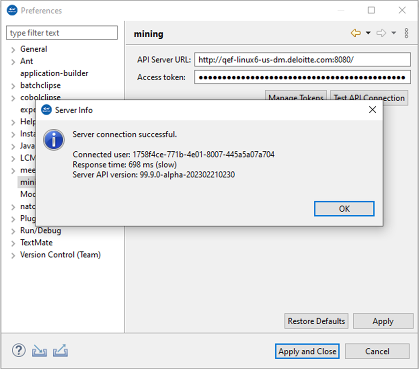
Option B: Connect without Keycloak
Step 1:
Enter the URL of the API server you wish to connect with, and then enter the access token ff93340a-af6c-4fcd-90bb-426448fa1597 in the Access token field.
Step 2:
Click Apply .
To check whether the connection to the server has been established, you can click Test API Connection . If the connection exists, the “Server connection successful” message will be displayed. The message also shows the connected user, the response time, and the server API version.
Step 3:
Click Apply and Close .
Logging
Logging helps you verify that the Eclipse-based tooling and server connection are working as expected. The sections below show where Mining writes diagnostic information and how you can review it inside the IDE. Use these logs first when you need to investigate warnings, errors, or connectivity issues.
Workspace log
Logs are written to the Workspace Log. It is located in your Eclipse workspace in the .metadata folder and is named .log.
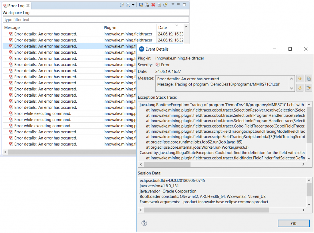
Error log view
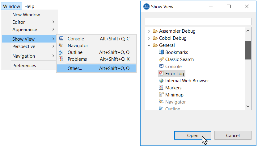
The error messages and warnings listed in the Workspace Log are also shown in the Error Log view in Eclipse. To display the Error Log, navigate to Window > Show View > Error Log and click Open .
To view details, double-click the corresponding entry.
User management without Keycloak - Information for system administrators
The following sections provide information for system administrators. They describe the built-in user and token model that is available when Keycloak is not part of the deployment. Use this information to review default access and to provision additional users in older or simplified environments.
User and OAuth access
The database schema comes loaded with an administrator (Username: admin) user with the following access token:
| admin user access token |
|---|
| 6c2000c1-d9a8-4d87-92f0-0a11139a037e |
If multiple miners will be using the Mining API server, additional users should be created according to the instructions in the section below.
Creating a new user
Warning
This section is for OrientDB only and is deprecated for the newest version of Code Discovery & Mining
Complete the following steps to create a new user:
Step 1:
Generate the user password hash by starting the Mining server with the argument "hashpw"
Step 2:
When prompted, enter the user password to hash. Find the hashed password in the next line.
Step 3:
In a web browser, enter the URL on which the database is running, followed by a colon, followed by the port (always 2480), for example. localhost:2480.
Step 4:
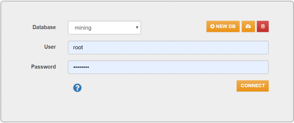
In the window that opens:
-
For Database, select mining from the drop-down list
-
Enter the credentials of the database and root user
-
Click CONNECT
Step 5:
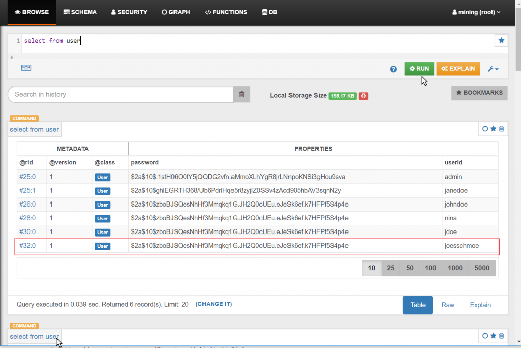
An OrientDB window opens. In the top field, create the new user by executing the following SQL with the new user name and the password hash that you created before.
Step 6:
Click RUN .
Step 7:
Verify the creation by running select from user. Now the user is displayed in the user table.
Creating the access token
Follow these steps to create an access token:
Step 1:
Create the access token by using the OAuth service with Postman as follows. On the landing page, click GET STARTED .
Step 2:
The download page will open. From the drop-down menu, select Windows 64-bit.
Step 3:
On the page that opens, beneath "Untitled Request", select POST from the drop-down menu and enter localhost:8080.
Step 4:
Navigate to the Authorization tab and select Basic Auth.
Step 5:
Navigate to the BODY tab and select the x-www-form-urlencoded radio button.
Successful result:
Step 6:
Use the provided access token in the mining-plugin preferences or on any mining-server call as url argument "access_token".
Example:
http://server:port/?access_token=f4be410d-996e-455d-b95e-19465d525ad9
Identity and access management IAM with Keycloak
The IAM feature allows administrators to manage user privileges by means of role-based access control (RBAC). While Identity Management covers authentication (for example, signup, login, password reset, etc.), access management deals with the authorization of the access levels to features in the Mining platform.
Authentication takes place via Keycloak. Keycloak is an external tool that is integrated into Mining. For more information, see the official Keycloak documentation at https://www.keycloak.org/docs/latest/.
Users can only be created via Keycloak; however, the user "Admin" ("god mode" admin) can access the page for creating users in Keycloak via the Global menu in the web UI (Global > Users).
Roles and definitions
The following table describes the available roles and access levels.
| Role | Description |
|---|---|
| Admin | The highest role in the user hierarchy, can also understood as "super user", "root", or "god mode". A general characteristic of admin role is that this role holds rights to manipulate data structures (for example, executing SQL commands). A user with a "admin" role has no restrictions and must be assigned to users wisely. |
| Client Admin | The Client Admin role provides similar rights to an Admin, but is scoped to a defined client. It can be understood as an Account Manager. Like the Admin role, one of the features of the Client Admin is the right to manipulate data structures of projects, such as modifying annotation categories or taxonomies. |
| Manager | The Manager role is provided for the project leads and allows manipulation of the mining baseline data. This is typically a person from the business function, that is, a person who is capable of understanding and approving the mined data. |
| Editor | Users with the Editor role have basic editing rights needed to work with Mining effectively, such as creating annotations, assigning taxonomies, creating descriptions, etc. |
| Viewer | The Viewer role is effectively a read-only role that can access and view features but can not add or modify data. This role is designed to allow an insight into the delivery and service process as a spectator, and to ensure that this user cannot edit data. |
Access matrix
The following matrix represents the various access levels and permissions.
| Project Nature | Client Admin (Restricted to specific client) |
Admin | Manager (Restricted to assigned project) |
Editor (Restricted to assigned project) |
Viewer (Restricted to assigned project) |
|
|---|---|---|---|---|---|---|
| Users | ||||||
| Assign "Admin" role (via Keycloak) |
n/a | ❌ | ❌ | ❌ | ❌ | ❌ |
| Assign "Client Admin" role | n/a | ✅ | ✅ | ❌ | ❌ | ❌ |
| Clients | ||||||
| See/Read | n/a | Only those clients from which projects the current user is assigned to | ✅ | ✅ | ✅ | ✅ |
| Add, Edit, Delete | n/a | ❌ | ✅ | ❌ | ❌ | ❌ |
| Projects | ||||||
| See/Read | n/a | All of specific client | ✅ | ✅ | ✅ | ✅ |
| Add, Edit, Delete | n/a | ✅ | ✅ | ❌ | ❌ | ❌ |
| Assign Members with Regular Roles (Manager, Editor, Viewer) |
n/a | ✅ | ✅ | ❌ | ❌ | ❌ |
| Override Project Nature on User (for example, access Mining features in a Discovery-only project) |
n/a | ❌ | ✅ | ❌ | ❌ | ❌ |
| Legacy Discovery Import | ||||||
| Server-side Import Discovery Excel/CSV Legacy |
Mining | ✅ | ✅ | ✅ | ❌ | ❌ |
| Discovery on Mining | ||||||
| Discover Code on selection |
Discovery Mining | ✅ | ✅ | ✅ | ❌ | ❌ |
| Discover Metrics on selection |
Discovery Mining | ✅ | ✅ | ✅ | ❌ | ❌ |
| Discover DNA on selection |
Discovery Mining | ✅ | ✅ | ✅ | ❌ | ❌ |
| Upload Source Code Files (Advanced) |
Discovery Mining | ✅ | ✅ | ✅ | ❌ | ❌ |
| Download Source Code Files (Advanced) |
Discovery Mining | ✅ | ✅ | ✅ | ✅ | ✅ |
| Upload Configuration (Advanced) |
Discovery Mining | ✅ | ✅ | ✅ | ❌ | ❌ |
| Download Configuration (Advanced) |
Discovery Mining | ✅ | ✅ | ✅ | ✅ | ✅ |
| Export Discovery Excel/CSV | Discovery Mining | ✅ | ✅ | ✅ | ❌ | ❌ |
| Export Summary Effort Excel | Discovery Mining | ✅ | ✅ | ✅ | ❌ | ❌ |
| Annotations | ||||||
| See/Read Annotations on Code | Mining | ✅ | ✅ | ✅ | ✅ | ✅ |
| Add, Edit, Delete Annotations on Code | Mining | ✅ | ✅ | ✅ | ✅ | ❌ |
| Set status to "Approved" | Mining | ✅ | ✅ | ✅ | ❌ | ❌ |
| Maintain Annotation Categories (project specific) | Mining | ✅ | ✅ | ✅ | ❌ | ❌ |
| Bulk Deletion | Mining | ✅ | ✅ | ✅ | ❌ | ❌ |
| Data Dictionary | ||||||
| See/Read Entries | Mining | ✅ | ✅ | ✅ | ✅ | ✅ |
| Add, Edit, Delete Entries | Mining | ✅ | ✅ | ✅ | ✅ | ❌ |
| Validate Text Selection | Mining | ✅ | ✅ | ✅ | ✅ | ❌ |
| Bulk Deletion | Mining | ✅ | ✅ | ✅ | ✅ | ❌ |
| Module Description | ||||||
| See/Read | Mining | ✅ | ✅ | ✅ | ✅ | ✅ |
| Edit/Delete | Mining | ✅ | ✅ | ✅ | ✅ | ❌ |
| Taxonomy | ||||||
| See/Read Taxonomies | Mining | ✅ | ✅ | ✅ | ✅ | ✅ |
| Add, Edit, Delete Taxonomies | Mining | ✅ | ✅ | ✅ | ❌ | ❌ |
| Assign, Bulk Assign / Propagate Taxonomy to Module | Mining | ✅ | ✅ | ✅ | ❌ | ❌ |
| Job Framework | ||||||
| See Jobs and Results | Mining | All of specific client | ✅ | ✅ | ✅ | ❌ |
| Cancel/Delete Job | Mining | All of specific client | ✅ | ✅ | ✅ | ❌ |
| Entity Meta Model (Custom Properties) | ||||||
| See/Read/"Use" properties | Mining | ✅ | ✅ | ✅ | ✅ | ✅ |
| Create/edit/delete properties | Mining | ❌ | ✅ | ❌ | ❌ | ❌ |
| Automated Analyses | ||||||
| Candidate Item Identification | Mining | ✅ | ✅ | ✅ | ❌ | ❌ |
| Technical Taxonomy | Mining | ✅ | ✅ | ✅ | ❌ | ❌ |
| Module Description | Mining | ✅ | ✅ | ✅ | ❌ | ❌ |
| GenAI | ||||||
| Bulk Generation of Annotation Descriptions | Mining | ✅ | ✅ | ✅ | ❌ | ❌ |
| Generate Single Reachability Block Description | Mining | ✅ | ✅ | ✅ | ❌ | ❌ |
| Bulk Generate Reachability Block Description | Mining | ✅ | ✅ | ✅ | ❌ | ❌ |
| Bulk Generate Module Description | Mining | ✅ | ✅ | ✅ | ❌ | ❌ |
| Reachability Analysis | ||||||
| Initiate Reachability Analysis | Mining | ✅ | ✅ | ✅ | ❌ | ❌ |
| Edit Name and Description of Single Reachability Block | Mining | ✅ | ✅ | ✅ | ✅ | ❌ |
| Activate/ Inactivate Single Reachability Block | Mining | ✅ | ✅ | ✅ | ✅ | ❌ |
| Merge / Un-Merge Reachability Blocks | Mining | ✅ | ✅ | ✅ | ✅ | ❌ |
| Bulk Inactivate Reachability Blocks | Mining | ✅ | ✅ | ✅ | ❌ | ❌ |
| Download CSV Data from RB Table View | Mining | ✅ | ✅ | ✅ | ✅ | ✅ |
| Dismiss Removed Reachability Blocks | Mining | ✅ | ✅ | ✅ | ✅ | ❌ |
| Sort Reachability blocks in Overview screen (Table View) | Mining | ✅ | ✅ | ✅ | ✅ | ✅ |
| Download Graph Views for Single Reachability Block | Mining | ✅ | ✅ | ✅ | ✅ | ✅ |
| Taxonomy Assignment to Modules within Reachability Blocks | Mining | ✅ | ✅ | ✅ | ❌ | ❌ |
| Recalculate Reachability Blocks | Mining | ✅ | ✅ | ✅ | ❌ | ❌ |
| Reveal Neighbors of Reachability Blocks | Mining | ✅ | ✅ | ✅ | ✅ | ❌ |
| Others | ||||||
| Initiate AST/Control Flow Calculation | Mining | ✅ | ✅ | ✅ | ✅ | ✅ |
| SQL REST-Endpoints | n/a | ❌ | ✅ | ❌ | ❌ | ❌ |
| Feature Console/Toggle | n/a | ❌ | ✅ | ❌ | ❌ | ❌ |
| Export (for example, CSV, Export Extensions) |
Mining | ✅ | ✅ | ✅ | ✅ | ✅ |
AWS Mining setup
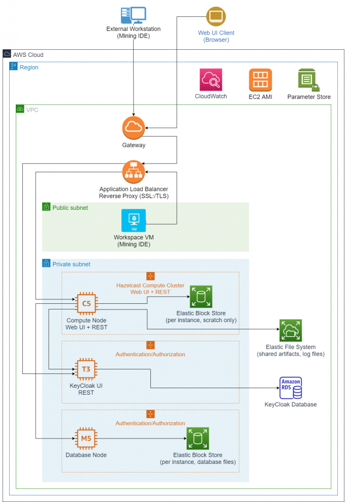
This chapter outlines the recommended setup and configurations for Mining with Amazon Web Services (AWS) components. The goal is to separate the API, database, identity, and shared storage layers so the environment can scale and be managed independently. The EC2 instances are designed to be launched from reusable machine images and connected through the AWS services listed below.
-
A cluster of EC2 instances with Elastic Block Stores (EBS) for Mining API servers
-
One or more EC2 instances with Elastic Block Stores (EBS) for the Postgres database
-
An Elastic File System (EFS) as a shared location for Mining server artifacts and logs
-
Auto Scaling groups to launch above EC2 instances as required from Amazon Machine Images
-
An EC2 instance hosting KeyCloak
-
An Application Load Balancer
AWS architecture diagram
The following diagram provides an overview of a suggested Discovery and Mining AWS setup:
Info
All compute node instances form one Hazelcast compute cluster with significant traffic between them. Auto scaling for KeyCloak is an option, but one instance is expected to be sufficient. The database cluster uses Hazelcast for replication across all nodes with significant traffic between them.
Mining IDE
Configuration
Java 11 or 17 (or higher) must be installed on the machine hosting the Mining IDE. The machine must be able to make a network connection to the Mining API server, KeyCloak server and Postgres database instances.
The Eclipse-based Mining IDE is delivered in the form of an archive file in ZIP format, which needs to be extracted.
The ZIP archive contains all of the necessary files and executables. As far as installation goes, this is the only step.
To start the Mining IDE, a user needs to log in to the machine and run the Eclipse executable, eclipse.exe.
The required innoWake.lic license file is bundled into the ZIP archive in the appropriate location.
When setting up a Windows machine image in AWS, it is recommended that the default TCP RDP port 3389 be open so a user can log in. The user will need the Administrator login and password from AWS to be able to log in at first. Afterwards, they can create additional users if needed.
The Mining IDE will connect to the Mining server and authenticate with the KeyCloak server. Therefore, it requires the proper Security Group configuration in AWS.
Keycloak server
Configuration
Java 8 (or higher) must be installed on the machine before starting the KeyCloak application, as it runs in the JVM.
The KeyCloak server is delivered in the form of an archive file in ZIP format, which needs to be extracted. The archive includes all necessary files and configurations needed.
To extract the file, transfer the archive file to the machine and run the following command via an appropriate CLI:
KeyCloak exposes the admin console UI on port 8080 by default. This port can be changed if needed by adjusting the following line in the file /standalone/configuration/standalone.xml:
Configuration
If port 8080 is changed it needs to be reflected in the Mining server’s Spring configuration. This configuration value can be passed in as an argument when starting the Mining server: --keycloak.auth-server-url=http://<url>:<port>/auth.
The ZIP archive includes a Mining theme and extension for the KeyCloak configuration, which need to be moved to dedicated locations:
-
Copy
mining-keycloak-theme-*.jarto/standalone/deployments/ -
Copy
mining-keycloak-extension-*.jarto/standalone/deployments/
The Mining theme needs to be selected manually once after setup via the KeyCloak Admin UI.
Start KeyCloak by executing the following command via an appropriate CLI:
Info
The standalone.bat/sh should start with the -b=0.0.0.0 parameter to allow non-local connections, that is, connections from another machine.
Warning
KeyCloak uses an embedded H2 (in-memory) database by default. While H2 can be persisted to disk it is highly recommended to connect this to a persistent RDBMS. KeyCloak’s documentation best describes this setup: https://www.keycloak.org/docs/latest/server_installation/index.html#_database The choice and setup of the RDBMS is left to the administrator.
A set of commands needs to be executed in the <KEYCLOAK-INSTALLATION-DIRECTOR>/bin directory to set up the server.
The following commands use default values for the admin user, password, and server port. Please adjust these appropriately where needed. The admin user needs to be set up manually so they will be able to log in to the KeyCloak UI and perform the configuration for any identity management integration.
Configuration
If these default values are changed, they need to be reflected in the Mining server’s Spring configuration. This configuration value can be passed in as an argument when starting the Mining server: --keycloak.auth-server-url=http://<url>:<port>/auth.
After this has been set up, the web application should be available by navigating to the admin console in a browser at <IP of KeyCloak server>:<port>/auth. Log in with the admin credentials used in the command above.
The Deloitte Mining product uses KeyCloak for most of its base functionality. For further details, please refer to KeyCloak's documentation (https://www.keycloak.org/documentation).
Single sign on (SSO)
Info
This section covers the basic setup for SSO. It is possible that further steps are required for your internal systems.
A proper SSL setup of the backend application is mandatory.
The following points need to be considered:
-
Self-signed certificates are prohibited.
-
A DNS record needs to be requested to acquire a public signed certificate.
-
On AWS, an application load balancer can provide SSL termination and a static URL.
-
The URL the SSO solution should redirect to after login has to be activated upon request.
-
The SSO administrator will then provide configuration parameters (for example, "client ID", "client secret"), which need to be specified in the KeyCloak Admin UI.
The SSO settings in KeyCloak itself can be configured entirely via the KeyCloak Admin UI.
Mining API server
Configuration
Java 17 must be installed on the machine before starting the application server, as it runs in the JVM.
The KeyCloak server is delivered in the form of an archive file in ZIP format, which needs to be extracted. The archive includes all necessary files and configuration needed.
To extract the file, transfer the archive file to the machine and run the following command via an appropriate CLI:
Inside the archive is the Java Spring Boot JAR and a Spring configuration file application-config.yml. The application-config.yml file needs to be updated with the correct IP addresses and ports for the Postgres database and the KeyCloak server. It also needs to be updated with appropriate performance settings based on the machine’s resources.
Settings to be modified in the Spring config are:
Warning
KeyCloak and the Postgres database must be up and running, configured, and available for connection before starting the Mining API server; otherwise, it will fail to start.
Start the Mining API server by executing the following command via an appropriate CLI:
Info
Percentages values here are based on the machine’s total memory, assuming the machine is dedicated to running this server. Example for a machine with 128GB total memory: -Xms50G -Xmx100G.
Example start command for a machine with 64vCPU and 128GB RAM
Alternatively, to the inline Spring configuration options, Deloitte can provide a default spring-configuration.yml file that can be bundled within the Mining API server zip file. This file contains the full properties used for Spring and can be modified as mentioned above. To use the Spring configuration file, adjust the jar command:
In addition, the server start can be set up as a service in a Linux system by creating a systemd service. This provides benefits like automatic restart and service control via systemctl.
Instructions for this step are intentionally left out, as it is within the administrator's discretion to configure system services.
Clustered Mining environment with AWS ASG
This section will outline the setup of a full-fledged auto-scaled Mining API server cluster on EC2, with full integration of the API server into the Auto scaling life cycle for graceful instance termination and central log and job result storage via an EFS (Elastic File System).
Simple Notification Service (SNS)
An SNS is required to enable the Auto Scaling group to send life cycle messages to the Simple Queue Service (SQS) queue created in the next step.
Step 1:
In the Amazon SNS Console, choose Topics and select Create Topic.
Step 2:
Type select Standard.
Give the topic a meaningful name click Create Topic to finalize the SNS setup.
Simple Queue Service (SQS)
A queue will be used by the Auto Scaling group to send life cycle notifications to be processed by the Mining API server instances.
Step 1:
In the Amazon SQS Console, select Create Queue.
Step 2:
Type select Standard.
Step 3:
Under Configuration, customize the SQS queue according to your needs.
Step 4:
Under Access policy, enter your AWS account number and the ARN of the IAM role that will be assigned to the EC2 instances.
Required permissions in addition to the default clustering permissions are "sqs:GetQueueUrl", "sqs:ReceiveMessage" and "sqs:DeleteMessage".
Step 5:
Apply further configurations as needed (for example, encryption). Then select Create Queue.
Step 6:
In the queue overview page, select Subscribe to Amazon SNS topic and select the previously created SNS topic.
Elastic File System (EFS)
An EFS (Elastic File System) storage mounted into each EC2 instance enables us to store all log files created by all instances at a central location, even after they are terminated.
A centralized EFS for logging is required for Discovery if the API server is clustered. This way the log files can be returned to the Mining IDE once a code scanning job has finished.
Step 1:
Create a dedicated EFS and customize it according to your needs (automatic backups, life cycle management, encryption, etc.).
Step 2:
For the network access settings, ensure that the same subnet is selected that will also be used by your cluster or Auto Scaling setup. Otherwise, the EC2 machines won't be able to mount the EFS storage. Remove the default security groups that may have already been applied, and select a security group that is different from the one that will be used for the EC2 instances.
Info
The security group used for the EFS needs an inbound rule that allows NFS traffic with the source being the security group used for the EC2 machines. While the security group for the EC2 machines needs an outbound rule allowing NFS traffic with the destination being the security group of the EFS.
Info
An EFS storage can be mounted in different ways. Choose your created file system and click Attach to see the possible commands. When mounting via DNS you have to make sure that DNS lookups are enabled and working in your VPC.
Amazon Machine Image (AMI)
Every machine started by the Auto Scaling Group will use the same AMI that must already contain all required resources for the machine to participate.
Step 1:
Set up a machine as described above in the Mining API Server.
All resources must be copied to the instance, like the Mining API server jar, application config YML, and log4j configuration. The application config must contain the following properties:
tagKeyandtagValuethat contain a unique key and value pair to make sure that only machines using the same key/value pair are eligible to form a cluster (the values chosen here are required later on when creating the launch template). Use a meaningful value, especially fortagValue.
Warning
If you do not set this tag, then all api-server instances on all machines in the region of your AWS account will be used to form a cluster, which is not recommended for this Auto Scaling setup.
-
lifecycleQueueName: Provide the name of the SQS queue created previously. -
jobResultFolder: Since all job results should be stored in the centralized EFS storage, provide the path of the mount point where the EFS storage will be mounted to during the EC2 instance launch. -
logFolder: Since all logs should be stored in the centralized EFS storage, provide the path of the mount point where the EFS storage will be mounted to during the EC2 instance launch.
Example configuration in YML application config
Step 2:
Provide any other AWS properties you may need for your setup as described in Mining Job API - AWS.
Step 3:
In the Amazon EC2 Instances Console, select the machine that you have set up. Choose Actions → Image and templates → Create image to create your Mining Server AMI.
Launch template
The launch template will be used by the Auto Scaling group to launch the EC2 instances.
Step 1:
Create a Launch Template for the AMI created above.
Step 2:
For Resource tags, add the following, while making sure to set Resource types to both Instances and Volumes:
-
Key="Name" and Value="
". -
Additionally the
tagKeyandtagValuepair that you already entered in the application config above during your AMI setup. Based on the example above Key="api-server-cluster" and Value="mining-autoscaling-cluster"
Step 3:
For Advanced details, set the following:
-
IAM instance profile should be set to the cluster and SQS-capable IAM role used during the SQS queue creation.
-
In User data, enter everything that should be executed when a new EC2 instance is launched.
Example Java launch command for the Mining API server
This installs the Amazon EFS utils, creates a mount point, actually mounts the EFS storage, and changes the owner of the mount point to ensure that the API server can write to the mount point. The mount point used here is "/mnt/efs", as already configured in the application config above. The IP "10.195.130.75" for the mount command should be replaced with the IP of your previously created EFS storage.
Finally, we switch to the directory that contains all Mining API server resources and execute the Java command to start it. The example above expects an explicit log4j2 configuration to be present in this location, along with the spring configuration file.
Step 4:
Finalize the launch template by customizing it according to your needs.
Load balancer
Before creating the Auto Scaling group, we will create a load balancer. Technically, this could also be directly created as part of the Auto Scaling group creation, but this way more fine-grained configuration can be done.
Step 1:
Create an Application Load Balancer and configure the name, scheme, HTTP port, availability zones with subnets, and security groups according to your needs.
Step 2:
Give the target group a descriptive name, set Target Type to Instance, set the protocol to HTTP, and the port to the one where your API server is configured to listen on (8080 by default).
Step 3:
Don't register any target and directly click Next: Review, and finally Create.
Auto Scaling Group
The final step is to create the Auto Scaling group for the Mining API server cluster.
Step 1:
Create an Auto Scaling group and choose the launch template created in the previous steps. Make sure to select Latest for the Version. This way, the auto scaling group will always automatically pick up the latest changes made to the launch template. Then click Next.
Step 2:
For Network, select the same subnet chosen during the load balancer creation.
Step 3:
Select Attach to an existing load balancer and choose the one created in the previous step.
Step 4:
Check Enable group metrics collection within CloudWatch and click Next.
Step 5:
Enter the capacities for your Auto Scaling group in the Group size section. Make sure that the Desired capacity and Minimum capacity should have a minimum value of 1. Otherwise, no machine will be started.
Keep Scaling policies at None and click Next.
Step 6:
Click Add Notification and select the SNS topic created in the previous step.
Step 7:
Finalize the creation of your Auto Scaling group by customizing it according to your needs, for example, with additional tags.
Step 8:
Create the policies that decide when to scale out/in the number of possible machines in the Auto Scaling group.
Ensure the following settings when creating policies:
-
For the Policy type, select Simple scaling.
-
Either use an existing CloudWatch alarm or create a new one.
-
To take the action, select Add 1 capacity units for the scale-out policy and Remove 1 capacity units for the scale-in policy.
Warning
Whatever type of policy you define, you have to make sure that your policy never reduces more than 1 machine per execution. This ensures that no more than one machine is being terminated at a time. Otherwise, the Hazelcast cluster may get into a corrupt state. Data may be corrupted when two machines are being terminated that both hold the primary and backup copies of a specific data structure.
Step 9:
Create the life cycle hooks that will send the life cycle events of the Auto Scaling group to your SQS queue, so that the API server can react. The type of life cycle hooks required cannot be created from within the AWS management console, but only from a Command Line Interface (CLI).
Access one of the EC2 instances initialized by the Auto Scaling group via SSH, open a CLI and and enter the following two commands to create two life cycle hooks.
The first command is for the EC2_INSTANCE_LAUNCHING event when additional instances are about to be launched, while the second one handles the EC2_INSTANCE_TERMINATING event when an instance is no longer required and should be terminated.
Replace the command parameters:
-
<your-life cycle-hook-name>: How the life cycle hook should be called. For example, "Launch_Api-Server_Instance" and "Terminate-Api-Server_Instance". -
<your-autoscaling-group-name>: The name of the Auto Scaling group created above. -
<your-SQS-queue-ARN>: The ARN of the SQS queue created above. -
<IAM-role-ARN>: The ARN of an IAM role that must have a trust policy to the EC2 Auto Scaling Service and the permissions "sqs:SendMessage", "sqs:GetQueueUrl", and "sns:Publish". This must not be the same IAM role that is used by the EC2 instances of the Auto Scaling group or the commands will not succeed. -
<your-region>: The AWS region.
In the Auto Scaling group console, select your group and navigate to Instance management. You should now see the two created life cycle hooks attached to the Auto Scaling group.
Step 10:
In the Amazon SQS Console, select your queue and click Send and Receive Messages.
Select Poll for messages, and you should see at least two messages that have automatically been sent during the creation of the life cycle hooks for testing purposes.
Step 11:
Your Auto Scaling environment is now set up.
You can access the Mining UI and attach the Mining IDE to the Mining API server via the DNS name assigned to the load balancer.
Example specifications
Mining API server
Component
Specifications
EC2 Linux AMI
-
c5.12xlarge (pre auto scaling)
- 48vCPU, 96GB memory
-
c5.12xlarge (pre auto scaling)
- 16vCPU, 32GB memory
EBS
-
gp2
-
100GB
Security Group
- Port 8080: HTTP requests in VPC (For Mining IDE, KeyCloak, Postgres, Users, etc.)
Keycloak
Component
Specifications
EC2 Linux AMI
- t3a.large
- 2vCPU, 8GB memory
Amazon RDS for PostgreSQL
- db.t3.medium
- 2vCPU, 4GB memory
EBS
-
gp2
-
100GB
Security Group
-
Port 8080: HTTP requests to the admin console for configuration
-
Other ports may be necessary for SSL, SSO redirect, etc.
Mining IDE
Component
Specifications
EC2 Windows AMI
- m5.2xlarge
- 8vCPU, 32GB memory
EBS
-
io2
-
150GB
-
5,000 IOPS
-
needed for storing source code files and moving them to the workspace
Security Group
-
Port: 3389 for RDP (Remote Desktop) access
-
Needs to be able to connect to Mining API server and KeyCloak server
OrientDB (deprecated)
Component
Specifications
EC2 Linux AMI
- m5d.8xlarge
- 32vCPU, 256GB memory
Instance store
- 2 x 300GB, NVMe SSD
Security Group
-
Port 2480: HTTP requests in VPC
-
Port 2424: All requests from Mining API server, none otherwise
Backups
- Scheduled job that exports the database to a dedicated S3 location
EFS
-
Standard Storage 350GB/month.
- Can be modified to configure infrequent access if needed to reduce costs.
-
Used for commonly mounted logging locations of the various services (Postgres logs, Mining API server logs, KeyCloak, etc.).
- This needs to be configured for each application to write its logs to this common mounted location instead of a local EBS or instance storage.
S3
- Standard Storage 300GB/month.
- Can be modified for the POST/GET requests count.
Approximate monthly cost estimate
Based on the AWS Pricing Calculator (https://calculator.aws/), using:
-
Pricing Model: EC2 instance savings plan
-
Reservation Term: 1 year
-
Payment option: No Upfront
| Mining Service | AWS Service | Type/Size | Monthly Cost (as of 01/2021) |
|---|---|---|---|
| Mining API Server | EC2 | c5.9xlarge | $700 |
| Mining API Server Storage | EBS | gp2, 100GB (x2) | $20 |
| KeyCloak Server | EC2 | t3a.large | $35 |
| KeyCloak Server Persistence | RDS | db.t3.medium | $50 |
| Common Logs | EFS | 350GB | $105 |
| DB Backup Storage | S3 | 500GB | $10 |
| OrientDB (deprecated) | EC2 | m5.8xlarge | $830 |
| Total | $1,750 |
Mining Job API
The Job API provides the backbone for executing specific operations as jobs that can parallelize operations into different tasks. When the Mining API Server is set up as a cluster, these tasks are automatically distributed for parallel execution.
Configuration
The following excerpt of a Mining API Server application configuration YML file shows the default job-api configuration. Use it as the baseline for standalone setups before enabling cluster-specific behavior. The property descriptions below explain which values are required for naming, logging, and shared job result storage.
The following configuration properties are available for the Spring application:
Parameter
Description and Values
name
The name that should be assigned to the cluster. Only mining-api-server instances having the same cluster name are eligible to join a cluster.
mode
The actual execution mode. The default value is standalone.
Valid values are:
-
standalone:This is the default setting when not explicitly providing amodeand will not create any cluster. -
default:The default cluster mode, which can be used to create a cluster based on the TCP-IP or Multicast configuration. -
aws:The cluster mode must be used together with the AWS-specific configuration to create a cluster on AWS.
nodeNameStrategy
The strategy is to assign a name to the cluster node, which can also be accessed in the log configuration. The default value is hostname.
Valid values are:
-
random-uuid:Every application startup will assign a new random UUID as the node name. -
internal-node-id:Assigns the Hazelcast member node ID, which will change with every application startup. -
ip:Uses the primary outbound IP address of the system. -
hostname:The default strategy uses the hostname of the local system. -
ec2-instance-id:When running on EC2, this uses the EC2 instance ID.
logFolder
Configures the base directory where all log files should be written to. Defaults to the logs directory where Java is currently running.
logFilePrefix
The prefix for all job-specific log files. The default value is job-.
jobResultFolder
Configures the base directory where the result files of Jobs are written to. Defaults to the jobResults directory where Java is currently running.
Warning
The logFolder and jobResultFolder must be accessible by all nodes of a cluster. Therefore, when running in clustered mode, these two properties must point to a shared file storage like an EFS on AWS.
Info
All properties with the exception of name are optional.
Multicast
Multicast is the easiest approach to create a cluster, but it may not be possible in all network environments.
Parameter
Description and Values
port (network)
The local port to use for the current process. Defaults to 5701 when not provided.
portAutoIncrement
When set to true the port will be automatically incremented until reaching one that is not already in use. Otherwise startup will fail. Defaults to true when not provided.
enableLoopback
If this is set to true then the loopback interface of the machine will be treated as a valid network interface during the node discovery. Defaults to false when not provided.
group
The address on which to send and receive multicast packets. Defaults to 224.2.2.3 when not provided.
port (multicast)
The port on which to send and receive multicast packets. Defaults to 54327 when not provided.
connectionTimeout
The time in seconds a node will wait for a multicast response from a different node before assigning itself to a master of its own cluster. Defaults to 2 when not provided.
ttl
The TTL of the multicast packets. Every hop between different networks decrements this value. Defaults to 32 when not provided.
trustedInterfaces
A comma-separated list of IPs that are eligible for the multicast lookup. When not provided, all machines available in the network are eligible to be included in the cluster.
Info
All mining-api-server instances with the same name property (for example, "my-cluster" as above) will be included in the same cluster by the multicast discovery process.
TCP-IP
In most network environments, the TCP-IP configuration is recommended if multicast is not available.
Parameter
Description and Values
port
The local port to use for the current process. Defaults to 5701 when not provided.
portAutoIncrement
When set to true the port will be automatically incremented until reaching one that is not already in use. Otherwise startup will fail. Defaults to true when not provided.
connectionTimeout
The time in seconds to wait for a response from one of the configured cluster members before giving up. Defaults to 5 when not provided.
members
A comma-separated list of IPs of all members that should participate in the cluster.
AWS
Creating a cluster on AWS is supported for EC2 machines (with and without Auto Scaling).
Parameter
Description and Values
`accessKey`
`secretKey`
Access and secret keys of your AWS account. If not set, iamRole is used.
`region`
The region where members are running. Default is the current region.
`hostHeader`
Either ec2, ecs, or the URL of an EC2/ECS API endpoint. Automatically detected by default.
`portRange`
A range of ports to locate members in the format <lower-port>-<upper-port>. The default value is 5701-5708.
`connectionTimeout`
readTimeout
The connection and read timeouts in seconds when making a call to the AWS API. The default value is 10.
`connectionRetries`
Number of retries while connecting to the AWS API. The default value is 3.
Info
All of the AWS and EC2 configuration properties are optional. If none of them have been provided, then the IAM role assigned to the EC2 instance will be used to form a cluster with all members running in the same region as that instance.
EC2
The IAM role needs to have the ec2:DescribeInstances permission to be able to form a cluster.
The following are EC2-specific properties, which must be contained in a ec2 subsection (all of these are optional):
Parameter
Description and Values
`iamRole`
The IAM role attached to the EC2 instance is used to fetch credentials if accessKey/secretKey is not specified. If not set, the default IAM role attached to the EC2 instance is used.
securityGroupName
The filter to identify only EC2 instances with the given security group.
`tagKey`
`tagValue`
The filter to identify only EC2 Instances with the given tagKey/tagValue.
Info
All of the AWS and EC2 configuration properties are optional. If none of them have been provided, then the IAM role assigned to the EC2 instance will be used to form a cluster with all members running in the same region as that instance.
EC2 Auto Scaling
The Job API is fully integrated into the AWS EC2 Auto Scaling life cycle.
In addition to the default EC2 configuration properties mentioned above, the following additional parameters can be adjusted for Auto Scaling:
Parameter
Description and Values
`lifecycleQueueName`
The name of the SQS (Simple Queue Service) queue that will receive the life cycle hook notifications of the Auto Scaling group.
Info
This is a required parameter for Auto Scaling.
activeJobsTimeout
When the Job API receives a machine termination notification from the SQS queue, it will wait for this duration (in seconds) for all currently running jobs on this instance to finish, while no longer accepting new ones. If there are still active jobs after the timeout, the AWS Autoscaler will be notified to keep the EC2 instance running, transitioning it back into service, and it will also accept new jobs again. Please note that the value chosen here should be smaller than the default timeout of the life cycle hook attached to the Auto Scaling group in AWS.
The default is 60 seconds, which is also the minimum possible value.
membersShutdownTimeout
During the shutdown process, when no jobs are active anymore on this member, it will gracefully detach itself from the cluster. If this takes longer than the configured timeout (in seconds), it will notify the AWS Autoscaler to transition the instance back into service. Please note that when choosing too small a value, the EC2 instance will transition back into service, but can no longer accept any jobs or tasks, as Hazelcast is already in a shutdown state.
The default is 600 seconds, with 60 being the minimum possible value.
Info
The lifecycleQueueName parameter is a required non-optional parameter for Auto Scaling to avoid compromising the cluster integrity and losing data.
Logging
The aforementioned configuration properties logFolder and logFilePrefix can be used to influence the log behavior.
The Job API provides multiple system properties, pattern parameters for trace logging, and context variables that can be used in the log4j configuration. These are:
System Property
Description
`job-api.cluster.nodeName`
Contains the resolved name of the cluster node as resolved by the configured nodeNameStrategy .
`job-api.log.logFolder`
Contains the final resolved log directory, which depends on the mode configuration property. In standalone mode, it will contain the raw value as provided in the logFolder configuration property, while in any cluster mode, is comprised of the logFolder configuration property and the cluster node name <logFolder-property-value>/<resolved-node-name>.
`job-api.log.logFilePrefix`
Contains the value of the logFilePrefix configuration property as-is.
Pattern Parameter
Description
`traceId`
Provides the ID of the current active tracing.
`spanId`
Provides the ID of the current active span.
`parentId`
Provides the ID of the parent span.
Context Variables
Description
`job-id`
Provides the ID of the job or task that triggered the log output.
Info
All system properties are populated at the earliest possible time when Spring actually creates the beans of the Job API. They are therefore not yet present during the Spring core initialization.
Configuration
When running in a clustered environment, the logFolder configuration property should point to a shared file storage like an EFS on AWS.
The following is a best practices example log4j2 configuration that shows how to use these properties and parameters:
The main point of interest is routing configurations. With these, one can achieve conditional logging depending on specific system properties or context variables.
The RollingFile Routing will create a log routing based on the job-api.log.logFolder system property. This is the main log file.
If the system property has not yet been set, all logs will be routed to the NullAppender appender, but are still handled by the Console appender as that is listed in the Root logger. You can also use a different appender in case these should be logged to a fixed file instead. If the system property has been set during the Job API initialization, then all log output is handled by the default Route below.
In this example, a RollingFile appender is used that receives its unique name based on the job-api.cluster.nodeName system property containing the cluster node name. It uses the job-api.log.logFolder system property to define the log directory. Depending on the configuration mode, the log file location will be resolved to the following:
-
In
standalonemode:<logFolder-config-value>/job-api.log, that is.logs/job-api.logwith the default configuration. -
In any cluster mode:
<logFolder-config-value>/<resolved-node-name>/job-api.log, that is.logs/my-hostname/job-api.logwith the defaultlogFolderconfiguration andnodeNameStrategyresolving the node name tomy-hostname.
Additionally, it showcases how to use the trace logging pattern parameters via %X{traceId}, %X{spanId} and %X{parentId}.
The job Routing shows how to route log output based on the job-id context variable. The logic closely resembles the RollingFile Routing, with the difference that it interacts with the context variable instead of the system property. This context variable is set by every job being executed, which enables you to separate the log output created by the job and its tasks into separate log files in addition to the main log file. Depending on the configured mode the log file location will be resolved to the following:
-
In
standalonemode:<logFolder-config-value>/<logFilePrefix-config-value><job-id>.log, that is.logs/job-1234.logwith the default configuration. -
In any cluster mode:
<logFolder-config-value>/<resolved-node-name>/<logFilePrefix-config-value><job-id>.log, that is.logs/my-hostname/job-1234.logwith the defaultlogFolderandlogFilePrefixconfiguration andnodeNameStrategyresolving the node name tomy-hostname.
REST endpoints
There are currently four REST endpoints located in JobController that can be used to request job information, their results, or to cancel them. Those endpoints are also documented through the Swagger UI (for example, when running the API server locally, http://localhost:8080/swagger-ui.html#/job-controller/).
| Method | URI | Parameter | Status Code | Description |
|---|---|---|---|---|
| GET | /api/v1/jobs | query |
200 | This endpoint can be used to get the JobInformation of all jobs that match the provided RSQL query. See below for more details on RSQL. |
| GET | /api/v1/jobs/{jobId}/info | jobId |
200, 404 | This endpoint returns the JobInformation of the job with the provided UUID. Status code 404 is returned if the job does not exist. |
| GET | /api/v1/jobs/{jobId}/cancel | jobId |
200, 404 | If the job produced a result like a CSV file or a job-specific Object, then this can be queried with this endpoint. This endpoint supports dynamic MIME type handling, depending on the information provided by the job implementation. Status code 404 is returned if the job does not exist. Status code 204 is returned if the job has no result. |
| GET | /api/v1/jobs/{jobId}/result | jobId |
200, 404, 204 | If the job produced a result like a CSV file or a job-specific Object, then this can be queried with this endpoint. This endpoint supports dynamic MIME type handling, depending on the information provided by the job implementation. Status code 404 is returned if the job does not exist. Status code 204 is returned if the job has no result. |
| GET | /api/v1/jobs/{jobId}/log | jobId |
202, 404, 403 | This endpoint returns the String representation of JobLog that matches the provided jobId if the user is authorized to access the job. Status code 404 is returned if the job does not exist or if the JobLog is empty. Status code 403 is returned if the user is not authorized to access the job. |
Info
The parameter jobId is a path variable containing the UUID of the job, while query is a request parameter.
Info
Status code 404 is returned if the requested job does not exist. Status code 204 is returned if the requested job has no result.
Code Discovery
Code Discovery
In this chapter, you'll learn how to initiate the Code Discovery process. The platform automatically identifies and categorizes code by programming language and type, giving you a comprehensive overview of your application portfolio. You will see an application view that highlights overall complexity, executable source files, and dependencies. Additionally, Mining helps ensure your application code is complete and verifies that it can be executed successfully.
Before you start, complete the Pre-discovery workflow to validate the source inventory, encoding, file layout, and language-specific prerequisites before the first Discovery run.
Preparatory steps
Before you can run Discovery, finish the Pre-discovery workflow and then perform the following preparatory steps. These tasks make sure your source modules, project linkage, and server connection are in place before analysis starts. Completing them first reduces rework later when you configure or execute Discovery.
Step 1:
Begin by importing the source modules. If there is already an existing Eclipse project with the legacy project nature, you can import it with the import wizard. Simply select Import... from the context menu and then, in the window that opens, select Existing Projects into Workspace. Otherwise, you must create a new project and add the client source modules.
Configuration
Note that Natural sources need to be extracted from the mainframe in SYSTRANS format using the SYSOBJH utility.
Step 2:
Ensure that you are connected to a mining server (see Mining API Server Connection).
Step 3:
If the target client or project does not exist yet, create it in the Mining web UI before you continue.
Step 4:
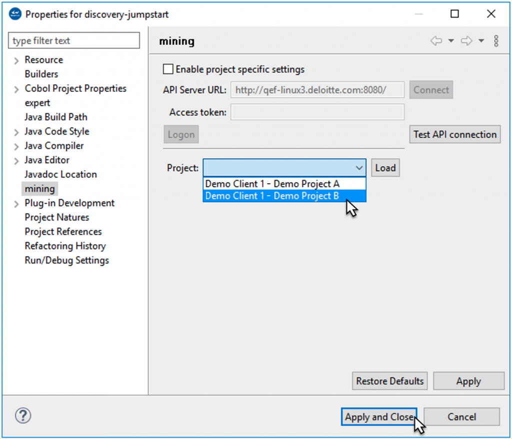
Use the context menu of the project to link the Eclipse project to a mining project on the API server. To do so, right-click the project, choose Properties > mining from the context menu, and then select your desired project from the drop-down menu. Click Apply and Close to complete the action.
Step 5:
After completion of the above steps, you can move on to configuring and executing Discovery.
Discovery configuration
This section introduces the Discovery configuration workflow and the options available to you.
You will learn when the default configuration is sufficient and when a customized Discovery_Config.xml is the better choice.
Use the following subsections to download, adjust, and apply configuration files before running Discovery.
Update the configuration before Discover Code
Download, edit, and upload the configuration files before you run Discover Code when the source package, folder structure, search order, or language settings differ from the default behavior.
Discovery with default settings
If you choose to run discovery with the default settings, you will use a default Discovery_Config.xml file that is stored on the mining database.
Info
Optional: You can view this config file by right-clicking the project and selecting discovery > Advanced > Download Configuration from the context menu to download the Discovery_Config.xml file to the workspace.
Discovery with customized settings
Alternatively, you can customize the Discovery_Config.xml file and specify your desired settings. To do so, right-click the mining project in your Eclipse workspace and select discovery > Advanced > Download Configuration from the context menu to download the Discovery_Config.xml file to the workspace.
This will create several configuration files in the root of your project:
-
Discovery_Config.xml: the main configuration file -
discovery-search-order.xml: configures the order in which dependencies are resolved on complex projects -
utilities.xml: configuration of project-specific third-party utilities -
DNA_Sequencer_Config.xml,DNA_SimilarityProcessor_Config.xmlandDNA_LouvainRunner_Config.xml: configuration files for the DNA feature
Use the following guidance when deciding which files to update:
| File | Change it when | Typical outcome |
|---|---|---|
Discovery_Config.xml |
You need to change enabled languages, parser behavior, margins, extensions, folder retention, or output options. | Discovery processes the uploaded source with the updated defaults. |
discovery-search-order.xml |
Dependencies are ambiguous, copybooks or procedures resolve from specific libraries, Java spans multiple package roots, or same-named DB objects appear across schemas. | Discovery resolves dependencies against the correct targets. |
utilities.xml |
Project-specific utilities need special handling instead of showing up as ordinary missing dependencies. | Discovery can treat configured utilities differently during dependency processing. |
| DNA configuration files | You need to tune the DNA feature after Code and Metrics discovery are already stable. | DNA processing uses project-specific sequencing or clustering options. |
Configuration
By default, the configuration is synchronized automatically when selecting any of the other Discovery commands. To view and edit the latest configuration before triggering an action, it can be uploaded to the mining server by selecting the context menu discovery > Advanced > Upload Configuration.
Scope the upload package
Before the first upload, decide which folders belong in the Discovery scope.
- Exclude generated code, test-only artifacts, build output, vendor drops, duplicate deliveries, and other out-of-scope content from the selected source directories or upload archive.
- Keep only the source that should produce Discovery results for the target application landscape.
- If excluded content still affects dependency interpretation, record that gap in the source inventory before the first run.
- Apply the same scope rules again before any forced full upload.
Discovery_Config.xml
This is the main Discovery configuration file, which allows for configuration of a large number of options for both Discover Code and Discover Metrics:
Key settings quick reference
Use this table to decide which settings are worth reviewing before the first run.
| Setting | Default or common use | Change it when |
|---|---|---|
ENABLE |
All languages are enabled by default. | Disable languages that are not present to improve speed and reduce false positives. |
PARSER_TIMEOUT |
Language-specific. | Increase the timeout for very large modules or slow parser workloads. |
RETAIN_FILE_EXTENSION |
false |
Set to true when the original source extension must be preserved. |
cobol_ims_dependencies |
false |
Set to true when IMS programs, databases, or control blocks are part of the source landscape. |
| COBOL parser margin settings | Standard fixed-column layout. | Change the margins when COBOL source uses non-standard columns. |
retain_dir_structure |
true |
Set to false when you want to flatten the discovered directory hierarchy. |
exclude_utility |
Project-dependent. | Enable it when project utilities should receive special handling through utilities.xml. |
COBOL_PGM_ID_AS_NAME |
false |
Set to true when module names should come from the PROGRAM-ID paragraph instead of the file name. |
Mappings
The <mappings> section of the config allows specifying where Discover Code places files with a certain file name or file type. Regardless of the setting, identified files are always placed in a language-specific folder inside the "src" folder. For example, Cobol files are always placed underneath "src/cobol" and Java files are placed in "src/java". Mappings allow to customize whether additional sub-folders are created underneath this language-specific folder (→ see also the <retain_dir_structure> setting).
The default mappings create additional sub-folders based on the file type, that is, separate folders will be created for programs, jobs, copybooks, etc.
Properties
The <properties> section allows for tweaking language-specific properties. All languages support the ENABLE, PARSER_TIMEOUT and RETAIN_FILE_EXTENSION properties.
Common properties
ENABLE
The ENABLE property can be set to false to disable processing of a language entirely. It is mainly useful for Discover Code. Since Discover Code tries to guess the file type of the source files, disabling languages that you know for sure do not occur in the source base can greatly speed up the process and increase its accuracy. Nonetheless, the setting is also applied to Discover Metrics and can be useful to speed up the Discovery process.
When the "src" folder contains source files in a language that is disabled via the configuration and "Discover Metrics" is run, then these files are not processed and will show up on the "Undiscovered" Excel sheet.
PARSER_TIMEOUT
The PARSER_TIMEOUT setting configures the maximum time in seconds that is used to attempt to parse a file. If the file can not be parsed successfully within this threshold, then the Discovery of the file is aborted, and no metrics or dependencies will be collected for the file. A separate PARSER_TIMEOUT can be configured for each language.
RETAIN_FILE_EXTENSION
The RETAIN_FILE_EXTENSION setting determines whether Discover Code preserves the original file extension. When set to "false" (the default), then a language-specific extension is applied, for example, Cobol files will get a ".cbl" extension.
Settings for ASSEMBLER language
UNKNOWN_TOKEN_THRESHOLD
This setting applies to Discover Code only. Sets the percentage of unknown tokens that may be contained in the file. If the file contains more unknown tokens than the threshold, then the file will not be classified as "ASSEMBLER".
Settings for BINARY language
PRINTABLE_CHAR_THRESHOLD
This setting applies to Discover Code only. Sets the percentage of printable characters that may be contained in a file. If the percentage is lower than the threshold, then the file will be classified as "BINARY".
Settings for COBOL language
COPYBOOK_PIC_THRESHOLD
This setting applies to Discover Code only. Sets the threshold for certain strings that typically occur in a copybook. If a file contains more than the configured percentage, then the file is classified as a COBOL copybook.
COBOL_PGM_ID_AS_NAME
These settings apply to Discover Metrics only. Determines how mining Modules for Cobol programs are named. When set to "false" (the default), the name of the Module will be equal to the file name, for example, if the file name is "EXAMPLE.cbl", then the program will be named "EXAMPLE". When set to "true", the value of the PROGRAM-ID paragraph inside the program is used instead.
cobol_ims_dependencies
Enable this setting when IMS programs, databases, or control blocks are part of the source landscape. Review it before the first Discover Code run because IMS dependencies are not collected when it remains disabled.
COBOL parser margin settings
Before Discover Code, verify whether the source uses standard COBOL columns 1-6, 7, 8-72, and 73-80. If the source uses a client-specific layout, update the COBOL parser margin settings before the first run to avoid parse errors and unexpected language classification.
Settings for CSD language
CSD_PARSER_DUMPXML
This setting will be removed with WMIN-5350 and should not be used.
Settings for JCL language
STEP_NAME
This setting can be specified multiple times and applies to Discover Metrics only. Despite its name, this setting does not configure any step names. Instead, it identifies DD names where the associated data sets will be identified as JCL control cards.
DD_KEYWORD
These settings list some parameter keys on DD statements, which are then treated in some way.
Settings for NATURAL language
DECIMAL_CHARACTER
Sets the character that is used as the decimal separator in Natural source files. This needs to be configured properly to parse Natural files successfully.
INPUT_DELIMITER
Sets the character that is used as the Natural input delimiter. This needs to be configured properly to parse Natural files successfully.
LANGUAGE_CODES
Sets which natural language codes to use when resolving dependencies. The language code is used to replace ampersand characters (&) in references to language-specific objects (for example, maps, dialogs, helproutines, subprograms).
Settings for ORACLE language
CDO_PATTERN_THRESHOLD
This setting applies to Discover Code only. Sets the threshold for certain strings that identify a file as a CDO file. If the file contains more than the configured percentage, it will be classified as CDO.
SQLMOD_PATTERN_THRESHOLD
This setting applies to Discover Code only. Sets the threshold for certain strings that identify a file as an SQLMOD file. If the file contains more than the configured percentage, it will be classified as SQLMOD.
Settings for PL1 language
PL1_PARSER_MARGIN_START
Configures the first column in PL/I files that contains source code. The contents of columns before this are treated as comments. Setting this property correctly is important for successfully parsing PL/I files.
PL1_PARSER_MARGIN_END
Configures the last column in PL/I files that contains source code. The contents of columns after this one are treated as comments. Setting this property correctly is important for successfully parsing PL/I files.
PL1_PARSER_ANS
Configures the column that contains printer control characters for PL/I.
PL1_PARSER_OR_SYMBOL
This setting can be specified multiple times and allows for defining additional symbols for the "OR" operator (for example, "|", "∨").
PL1_PARSER_NOT_SYMBOL
This setting can be specified multiple times and allows for defining additional symbols for the "NOT" operator (for example, "!", "¬").
Settings for VMS language
FMS_PATTERN_THRESHOLD
This setting applies to Discover Code only. Sets the threshold for certain strings that identify a file as an FMS file. If the file contains more than the configured percentage, it will be classified as FMS.
DCL_PATTERN_THRESHOLD
This setting applies to Discover Code only. Sets the threshold for certain strings that identify a file as a DCL file. If the file contains more than the configured percentage, it will be classified as DCL.
Settings for JAVA language
INCLUDE_PACKAGES
The setting INCLUDE_PACKAGES contains the filter for the packages to be included.
-
An empty value means that all packages of the source folder should be included in the discovery
-
When a pattern is specified, then only matching packages and all compilation units, whose package declaration matches the include pattern, are included by the discovery
By default, only (and all) packages inside the source folder are analyzed. If you want to see dependencies on third-party libraries, you need to include their package names here.
EXCLUDE_PACKAGES
The setting EXCLUDE_PACKAGES contains the filter for the packages to be excluded.
-
An empty value means that no packages are excluded in the discovery
-
When a pattern is specified, then all matching packages and all compilation units, whose package declaration matches the exclude pattern, are excluded by the discovery.
Settings for ECL language
ECL_PATTERN_THRESHOLD
This setting applies to Discover Code only. Sets the threshold for certain strings that identify a file as an ECL file. If the file contains more than the configured percentage, it will be classified as ECL.
File detection types
The <file_detection_types> section allows us to determine the order in which Discover Code applies techniques for identifying file types. The "MAIN" type uses language-specific parsers to parse the contents of files. The "TOKEN" type looks for specific tokens (strings). The "DEPENDENCY" type looks for references to other files (for example, identifying a file as a copybook by the fact that it is being included by a program). The "EXTENSION" type identifies files by their existing file extension.
Usually, there is no need to change this setting.
Other settings
<retain_dir_structure>
This setting determines whether Discover Code preserves the original directory structure when copying identified files to the source folder. The language-specific source folder (for example, "src/cobol") will be prepended to the original directory structure, and the additional sub-folders configured in "
<exclude_utility>
This option enables special treatment of the Modules described in the "utilities.xml" file. When set to "false", utility processing is disabled, and references to utilities will be treated like any other kind of dependency (which effectively means that utilities will most likely show up as "MISSING" Modules, since they are usually not part of the code base). For some languages, setting this to "true" also enabled additional processing. For example, it enables the parsing of utility-specific control cards for JCL
The name "exclude" of this property might be misleading. Setting it to "true" actually enables special handling of the utilities. It is historically called "exclude" because the utilities are being excluded from regular dependency processing, receiving special treatment instead.
<collect_statements>
Whether Statements are collected during Discover Metrics. Disabling this may (slightly) speed up the Discovery process, but the "Statements" sheet in Excel will be empty.
<undiscovered_folder>
The name of the folder in the root of the project where files are moved by Discover Code when their file type cannot be identified. The default is "undiscovered-entities".
<output_format>
Set to "EXCEL" or "CSV" to automatically download the Discovery results after running Discover Metrics in the specified format. Note that, regardless of this setting, you can always download the results in any format through the "Export" page on Mining UI.
Settings for special DDs
The special DDs listed below are supported.
-
SYSDUMP
-
SYSABEND
-
SYSMDUMP
-
SYSUDUMP
-
SYSCHK
-
SYSCKEOV
If dependencies from these DDs need to be ignored, add a tag to Discovery_Config.xml with the DD_IGNORE_DEPENDENCY key as shown below.
To get the proper metrics, rerun a discovery on existing projects. If the incremental scan feature is enabled, it must be disabled while re-running the project(s) so that the new metrics include the required changes.
discovery-search-order.xml
The discovery-search-order.xml file is used to tell the Discovery how to resolve ambiguous dependencies. For example, if one program makes a call to another program named "FOO", but there are multiple programs available in the source code with the name "FOO", then the Discovery doesn't know which one is called. This situation arises very frequently in real-world data because the source code is often structured into several projects or libraries, many of which often contain programs, jobs, or routines with the same names. The dependencies between these projects or libraries are often defined through build scripts or configuration files, which may or may not be part of the source code. As of now, Discovery cannot automatically determine these inter-project dependencies, and therefore, it is usually required to manually configure a discovery-search-order.xml.
You can tell that you probably need to configure a search order if you see the message "Multiple possible candidates found" frequently in the Discovery error sheet. It indicates that Discovery was not able to determine the target of a dependency because there were multiple possible candidates. In such a situation, Discovery does not create any dependency and instead generates this error message to not provide incorrect information.
Please note that many languages (for example, Cobol, Natural, PL/I, ...) make use of "assembling" where the source code is pieced together from several files ("copybooks", "copycodes", etc.). It is often required to have a properly configured discovery-search-order.xml to assemble and parse those files successfully. Therefore, a high number of parse errors could also indicate that you need to configure the search order correctly.
Use the following decision guide when deciding whether a project-specific search order is required:
| Scenario | Configure search order? | Why |
|---|---|---|
| Java spans multiple project roots or package roots | Yes, always | Java dependency resolution depends on explicit package-root targets. |
| COBOL copybooks or JCL procedures live in separate libraries | Yes | Include and procedure resolution must point to the correct library first. |
| Multiple repositories contain same-named modules | Yes | Prevents ambiguous dependency resolution and repeated "Multiple possible candidates found" warnings. |
| Multiple DB schemas contain same-named objects | Yes | Use <contained-in> rules to disambiguate schema-level dependencies. |
| One self-contained project has no repeated module names | Usually no | The default search order is often sufficient for the first run. |
Basic search order configuration
The discovery-search-order.xml file can configure any number of search orders. For each <search-order> one <source> and any number of <target>s (at least 1) can be defined. When resolving a dependency (or looking for include files during assembling), the discovery processes the configured search orders from top to bottom. It matches the current file (the file declaring the dependency or the file currently being assembled) against the <target> specifications is evaluated from top to bottom. The discovery will consider only dependency candidates that match the current <target>. If no such candidates exist, then the next <target> is tried. If there are no more targets in the current search order, then Discovery tries to find the next search order where the current file matches the source. If no search order matched or no targets were found, the dependency remains unresolved.
The default search order configuration looks like this:
It defines a single <search-order> where that
Info
The * Wildcard matches one path segment or part of a file name. The ** Wildcard matches any number of path segments (0 or more).
Here is a typical example of the search-order configuration required to assemble COBOL files properly:
This configuration tells discovery to assemble Cobol programs (files ending in .cbl) in the sub-project "projectA" using copybooks (files ending in .cpy) from the same project. The same is configured for "projectB". You can imagine a similar configuration for other languages, for example, for configuring the "proclib" for JCL.
Info
The path patterns are always relative to the root folder of your Discovery project and always start with "src" (or a wildcard character).
Special configuration for Java projects
Java projects often require a special search-order configuration to resolve any kind of dependency correctly. The reason for this is that Java uses the folder structure to define "packages". The root of this package hierarchy is the source folder. By default, the folder "src/java" is treated as the root of the package hierarchy. However, when running Discovery on Java projects, you typically have multiple projects, each with its own source folder. For example, your source folders might look like this:
-
src/java/project-1/src/main/java -
src/java/project-2/src/main/java -
src/java/project-3/src/main/java
Here we have three projects, each with its own source folder. The root of the package hierarchy for each project is the "src/main/java" folder inside each project folder. In this situation, it is mandatory to configure a discovery-search-order.xml. When configuring the search order for Java projects:
-
the
<source>pattern defines the root of the package hierarchy - it must give the full path to the project's source folder without using wildcards, but must then use wildcards to match all.javafiles contained within -
the
<target>patterns define where to look for dependencies by giving the location of additional package roots. You must even include a<target>for the same project, if you want to resolve dependencies within one project.
Here is an example search order configuration for the above project constellation. Let's further assume that "project-1" depends on "project-2" and "project-2" depends on "project-3". So "project-1" must be able to resolve classes from "project-2" and "project-2" must be able to resolve classes from "project-3". The search order is configured accordingly:
Additional properties
The discovery-search-order.xml configuration has additional properties that can be specified to describe the source and target.
The following properties can be specified as below:
-
name: the name of the target module (currently supports exact match only, that is, no placeholders) -
type: the expected type of the target module -
path: the exact path of the expected target - can be used as an alternative to a pattern when no wildcards are being used -
contained-in: as a separate sub-element: describes the "parent" module of the expected dependency
When resolving dependencies of modules of type "COBOL_PROGRAM" with path pattern "src/test/cobol", this configuration specifies that the "SQL_TABLE" modules contained in the "TEST-SCHEMA" schema are considered first before all other targets are attempted.
Important: To link discovery dependencies correctly with the imported DB schema, you must proceed in the following order:
-
Import the DB schema
-
Configure search-order if necessary
-
(Re-)run Discovery
Discovery directory structure
At the beginning of a Mining project, before the first Discovery is executed, the project contains the sources that need to be analyzed. The Discover Code step then identifies and moves these sources into a predefined directory structure.
Some folder names are therefore reserved, and the following file naming conventions apply:
-
Discover Code moves all identified files into a directory called
src. Undiscovered files, that is, files that have yet to be analyzed, shall therefore not be placed in a directory with this name, since Discover Code can not be executed on thesrcfolder. -
Identified files are sorted into
src/<language>directories. By default, the original folder structure is preserved underneath that path. If the original file was a Cobol program located in a folder calledundiscovered/foo/bar, then it will be placed intosrc/cobol/foo/bar.
This behavior can be adjusted in the discovery_config.xml file. -
Files that can not be recognized uniquely in language, but a language can be assumed, are moved to a folder
/src/maybe/<language>/, withbeing replaced by the assumed language. -
Discover Code moves all unidentifiable files into a directory called
undiscovered-entities. This directory name is therefore reserved and should not be used to designate undiscovered files.
Configuration
The name of the src folder where successfully identified files are moved is predefined and cannot be changed. The name of the undiscovered-entities folder, however, can be changed via the discovery_config.xml file.
Cross-project Java dependency support
It is common for a Java code base to consist of multiple projects that have dependencies on each other.
By default, these dependencies are not captured during the Discovery. To enable support for cross-project Java dependencies, the discovery-search-order.xml file needs to be added and configured in the Mining project's root directory.
The default configuration looks as follows:
The source pattern attribute defines the path from which the Java class files need to be considered for examining any cross-project dependency. The target pattern attribute defines the path where these Java dependency classes exist. These settings are used for assembling source files, for instance, programs using copybooks, and for dependency resolving.
Example
The configuration below will pick each class inside the project "project1" and check if that class contains any reference (dependency) to another class that exists in the project "project2".
Consider the following example code for the classes "project2\in\example\MyClass2" and "project1\com\example\MyClass1":
The example configuration above will capture that the module MyClass1 has a cross-project dependency on in.example.MyClass2.
utilities.xml
Use utilities.xml when the project contains third-party or client-specific utilities that should receive special handling during Discovery instead of being treated as ordinary dependencies.
A typical workflow is the following:
-
Define the utility modules in
utilities.xml. -
Review
exclude_utilityinDiscovery_Config.xmlwhen you want Discovery to apply utility-specific handling. -
Upload the updated configuration before running Discover Code or Discover Metrics.
If utility modules continue to appear as missing dependencies, review both utilities.xml and exclude_utility together before rerunning Discovery.
Running Discovery
This section covers the execution of the following Discovery operations. Run these operations in sequence to move from source ingestion to technical analysis and similarity grouping. The summaries below explain what each stage produces so you can choose the right action for your project state.
-
Discover Code: Discovery starts with this step, in which the code base is scanned, analyzed, and reorganized by language and module type.
-
Discover Metrics: In this step, the discovered code is closely inspected and evaluated by content, dependencies, complexity, and other criteria to provide detailed charts and reports in the Metrics UI.
-
Discover DNA: The purpose of the DNA analysis is to find similar modules in a code base and group them. This allows us the measure how similar code is, find patterns, and, for example, accelerate mining and modernization.
To create these clusters, Discovery sequences the code base's DNA and compares each module's DNA sequence to calculate its distance. Modules with similar DNA, that is, small distances, are then bundled into clusters.
Configuration
All Discovery features, that is, Discover Code, Discover Metrics, and Discover DNA, trigger a source code upload. To improve the speed of uploads, only sources that have changed since the previous Discovery are uploaded in subsequent executions. To force a re-upload of the full code base, select the directories with the source modules, right-click them, and select discovery > Advanced > Upload Source Code from the context menu.
Source upload behavior
All Discovery actions trigger a source upload. Use the initial run to upload the full source set, and expect later runs to upload only changed files.
- Discover Code, Discover Metrics, and Discover DNA synchronize source changes before the remote job starts.
- Use discovery > Advanced > Upload Source Code when you renamed, split, or reorganized many files and want to force a full re-upload.
- Review the pre-discovery checks before forcing a full upload so the server receives the corrected package.
- When a file exceeds the 16 MB encoded content limit, Discovery prompts you to continue with the large-file upload, skip the file, or stop and correct the source package first.
- Exclude generated code, test fixtures, build output, duplicate deliveries, and other non-scope content before you trigger the upload so they do not create avoidable noise in
src/maybeorundiscovered-entities.
API and scripted uploads
Automation can use an approved API client or integration to upload the prepared source package instead of relying on the interactive Eclipse workflow.
- Use the same target Mining project, source selection, and uploaded Discovery configuration that you would use for an Eclipse-driven run.
- Apply the same pre-discovery exclusions before packaging the archive for automation.
- Confirm the server-side Discovery upload size limit when large archives are expected.
- Validate the first automated run the same way you validate a manual run: review the resulting
srclayout,undiscovered-entities,src/maybe, and the downloaded job log.
Discover Code
Info
Discover Code does not need to be performed on imported Natural sources. The natclipse importer already places the sources into their correct libraries within src/natural and adds the correct file extensions to the source files. Discover Code also does not need to be performed on imported Java sources because the system retains the source folder structure by default. For more information on this, please refer back to Special Configuration for Java Projects
At this first discovery step, the miner must have maximum information about the types of client sources.
The sources for some languages initially do not have identifying extensions (as Natural programs, for example, with .nsp). The discovery process attempts to identify the correct types with parsing.
For ambiguous source structures, this can result in many artifacts in the folders /undiscovered-entities or /src/maybe.
To improve discovery results, it is recommended to apply the correct extensions to the source artifacts so they can be distinguished uniquely for a type. Adequate extension can be set by users with specific language knowledge, or the modules can be sorted into the correct folder at /src manually.
The following table shows recommended extensions and folders for sources by language and type:
| Language | Type | Extension | Identification |
|---|---|---|---|
| Cobol | Program | cbl | accurate |
| Copybook | cpy | ||
| BMS | map | ||
| MFS | |||
| Batch | Job | job | |
| Proc | proc | ||
| Assembler | Program | asm | accurate |
| Macro | asm | accurate | |
| PL/I | Program | pl1 | |
| Mainprogram | pl1m | ||
| Copybook | pcpy | ||
| SubRoutine | pl1m | ||
| Natural | Program | nsp | |
| Subprogram | nsn | ||
| Subroutine | nss | ||
| Copycode | nsc | ||
| Map | nsm | ||
| Help | nsh | ||
| DDM | |||
| Data Area | |||
| Function | |||
| Text | |||
| Error Message | |||
| Class | |||
| CPM | |||
| Adapter | |||
| Dialog | |||
| REXX | |||
| C | Program | c | |
| Header | h | ||
| Function | |||
| Java | |||
| XML | xml | ||
| Binary | bin | ||
| VAX-VMS | DCL | ||
| FMS | |||
| VAX_MACRO | |||
| ORACLE | CDO_FILE | ||
| CDO_RECORD | |||
| SQLMOD | |||
| CSD | LIST | ||
| EXTRACT | |||
| Easytrieve | .ezt | ||
| IMS-Cobol | Program | ||
| Copybook | |||
| IMS-JCL | Job | job | accurate |
| Proc | proc | difficult | |
| IMS | Program Specification Block PSB | psb | |
| Database definition DBD | dbd | ||
| ARCHDEF | |||
| HDAMPARM | |||
| TDFXTRCT | |||
| TEMPLATE | |||
| BASIC | PROGRAM | ||
| SUB_ROUTINE | |||
| FUNCTION | |||
| OBJECT | |||
| C++ | Program | cpp | accurate |
| Header | hpp | accurate | |
| C# | CompilationUnit | cs | |
| Namespace | cs | ||
| Class | cs | ||
| PartialClass | cs | ||
| Struct | cs | ||
| Interface | cs | ||
| Enum | cs | ||
| Attribute | cs | ||
| Record | cs | ||
| Project | csproj | ||
| Solution | sln |
Complete configuration changes before Discover Code
Review and upload Discovery_Config.xml, discovery-search-order.xml, and utilities.xml before the first run or whenever the source package changes. Discovery uses the latest configuration stored on the server.
Once you have completed the preparatory steps and applied configuration settings, you can proceed with Discover Code. To do so, select the directories with the source modules, right-click them, and select discovery > Discover Code on Selection from the context menu. This step may take some time.
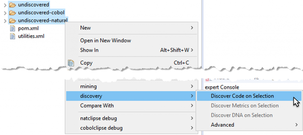
Info
To check the status/progress of Discover Code, open the Job View by selecting Window > Show View > Other from the Eclipse menu bar. Then type job view in the search field, select the Job View entry, and click Open. Now you can see the current state of the remote job, the elapsed and remaining time, and the result of the remote job.
Warning
Discovery will show a warning message for a file size limit of 16 MB per file. For this limit, the file content size after encoding is considered, not the file size stored on disk. When a source file with a content size larger than 16 MB is uploaded, a window will appear, and the user can click "Upload large files" to allow the discovery to continue. Otherwise, skip the large files or abort the process.
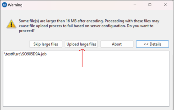
When the discover code job is finished, a job log file named discover-code-
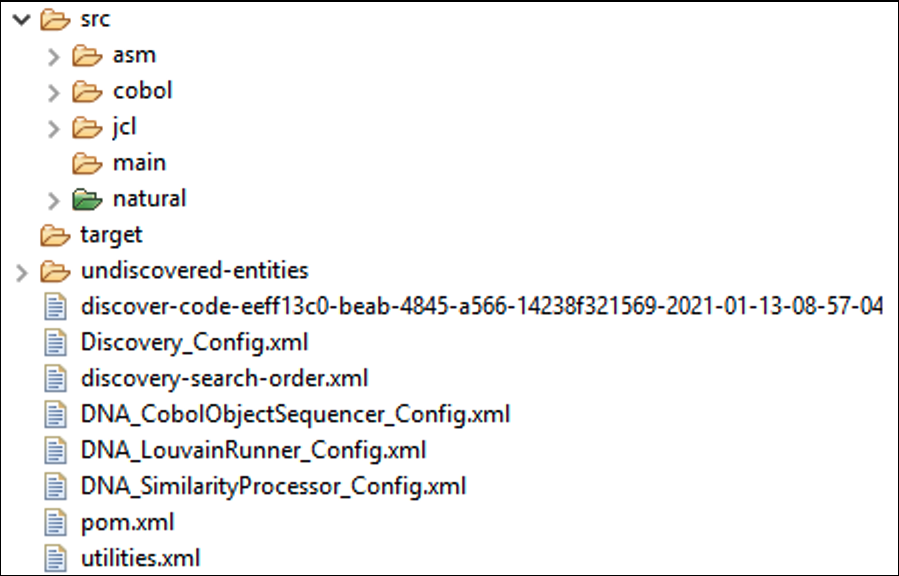
Configuration
It is possible to bypass source code upload when running Discover Code by holding down the Ctrl or Alt modifier key while selecting the option from the context menu.
After the first Discover Code run, review the results before continuing:
- Confirm that the expected languages and folder structure appear under
src. - Compare the discovered modules with your source inventory.
- Review
undiscovered-entitiesandsrc/maybe; they should be limited exception folders. - Open the job log to look for repeated parse failures, upload warnings, or ambiguous dependency messages.
- If the results do not match expectations, correct the source package or configuration and rerun Discover Code.
For common issues and rerun guidance, see Discovery troubleshooting.
Discover Metrics
Next, you can run Discover Metrics on the sources. To do so, right-click the src directory and select discovery > Discover Metrics on Selection from the context menu.
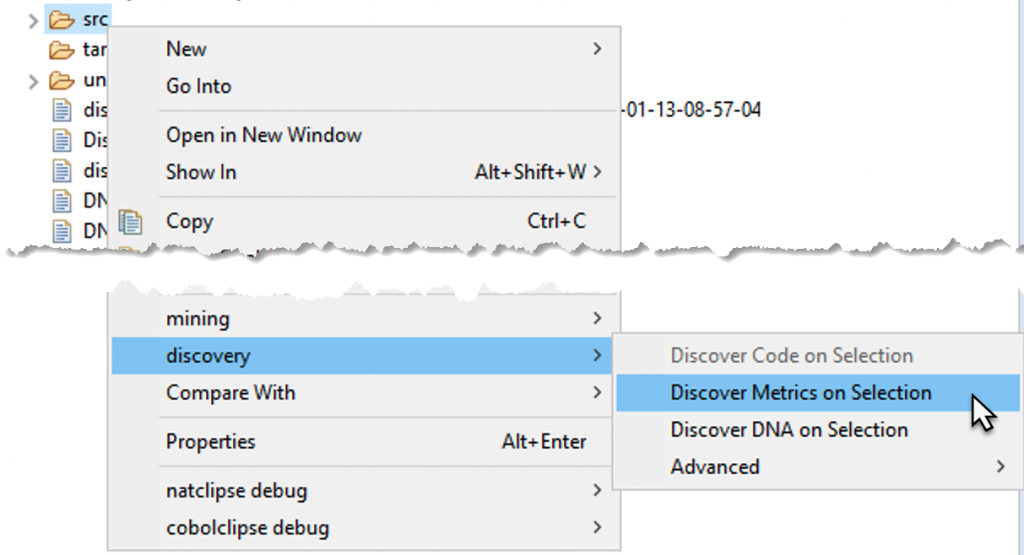
Info
The Job View displays the status/progress of Discover Metrics. It shows the current state of the remote job, the elapsed time, and the remaining time, as well as the result of the remote job.
When the Discover Metrics job is finished, a job log file named discover-metrics-
Info
The existence of a log file depends on the configured log level in the log4j2.xml file. For example, if the log level is set to OFF or ERROR, no log file is created when only INFO events are triggered.
The results of the Discover Metrics step are either downloaded as an output file named
-
discovery_<time stamp>.xlsxif you ran discovery with default settings, or -
discovery_<time stamp>.csvif you customized the discovery and changed the output format in the config file.
Another result of Discover Metrics is the effort-summary-<time stamp>.xlsx file. This file is also automatically downloaded to the workspace.
Rerun Discover Metrics after any change to extensions, margins, search-order rules, utilities, or source layout that affects module identity or dependency resolution.
Configuration
It is possible to bypass source code upload when running Discover Metrics by holding down the Ctrl or Alt modifier key while selecting the option from the context menu.
Configuration
On Linux hosts, the fontconfig package must be installed as a requirement for the Excel file generation.
Incremental vs full Discover Metrics scan
Discovery can be configured to perform incremental scans via the feature toggle incrementalScan in the Web UI feature console.
When enabled, repeated Discover Metrics executions will only rescan modules that have been changed (for example, LoC or metadata) and their dependencies, instead of rescanning the full code base.
To circumvent incremental scanning and force a full Discover Metrics scan, right-click your project's src folder and select discovery > Advanced > Force Full Discover Metrics Scan.
Forcing a full scan will also force a full source code upload.

Discover DNA
Configuration
Performing Discover Metrics is a prerequisite for Discover DNA. If modules are changed in the project, both processes should be re-executed to update the results.
Subsequently, you can run discover DNA. Right-click the src directory and select discovery > Discover DNA on Selection from the context menu.
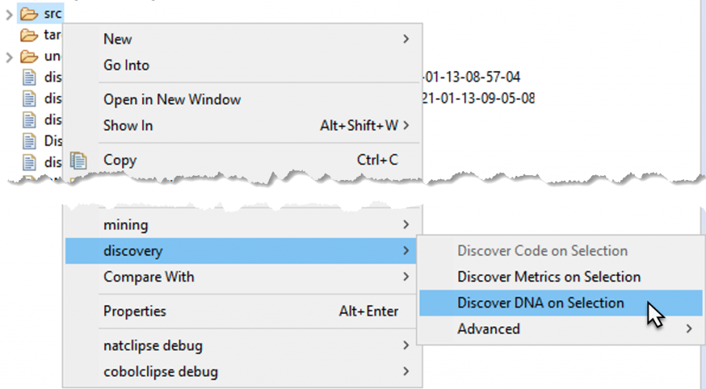
Info
The Job View displays the status/progress of Discover DNA. It shows the current state of the remote job, the elapsed time, and remaining time, and the result of the remote job.
When the Discover DNA job is finished, a job log file named discover-dna-<random id>-timestamp is automatically downloaded to the workspace.
Info
The existence of a log file depends on the configured log level in the log4j2.xml file. For example, if the log level is set to OFF or ERROR, no log file is created when only INFO events are triggered.
The results of the Discover DNA step can be downloaded from the Web UI by navigating to Exports > Download Modules in cluster. The downloaded file is a set of CSV files for each DNA type. The CSV file contains the list of similar modules, ordered by cluster ID.
Now you are ready to start mining. You can access the Web UI and find all the discovered modules in the project you selected in Preparatory Steps.
Pre-discovery workflow
Complete this workflow before you run Discover Code or Discover Metrics. It helps you validate the incoming source package, normalize files, confirm language-specific prerequisites, and decide which Discovery settings need to change before the first upload.
Source intake and inventory
Start with the source package itself. Discovery works best when the delivery method, folder layout, and expected content are documented before you import anything into Eclipse.
-
Obtain the complete source archive and record how it was delivered, for example, SFTP, a zip archive, or a repository clone.
-
Understand how the source is organized. Confirm whether development, test, and production artifacts share one tree or are split across separate repositories or folders.
-
Capture a source inventory that lists expected languages, module types, approximate counts, and known shared libraries.
-
Record source control and framework context, including proprietary build frameworks, shared utility libraries, scheduler definitions, or generated artifacts.
-
Document missing components before discovery starts, for example, missing copybooks, JCL procedures, DDL files, or schema definitions.
Warning
Discovery results can only be as complete as the source package that you receive. If the archive and the expected inventory do not match, resolve the gap before the first discovery run.
Identify languages and technologies
Compile the full list of languages and technologies present in the source package. This list drives your configuration, search-order, and pre-discovery decisions.
| Language or technology | Typical extensions | Verify before discovery |
|---|---|---|
| COBOL | .cbl, .cob, .cpy |
Copybooks are present, margins are known, and IMS usage is identified. |
| CICS | Embedded in COBOL | EXEC CICS usage is identified and supporting maps or copybooks are included when they are part of the source package. |
| PL/I | .pli, .pl1 |
Margin boundaries and custom OR or NOT symbols are known. |
| Natural | .nsp, .nsl, .nsa |
Files were extracted in SYSTRANS format and locale settings are known. |
| JCL | .jcl, .job, .proc |
Jobs, procedures, and in-stream data are split into separate files. |
| Java | .java |
Package roots are clear and multi-project dependencies are mapped. |
| C and C++ | .c, .h, .cpp, .hpp |
Shared headers and platform-specific dependencies are accounted for. |
| C# | .cs, .csproj, .sln |
Solution layout and .NET-specific source dependencies are identified. |
| SQL and DDL | .sql, .ddl |
Auto-margin detection and DB schema import requirements are understood. |
| Assembler | .asm, .s |
Threshold-based language detection is reviewed if token noise is expected. |
Validate and sanitize source files
Normalize the files before you upload them. This reduces misclassification, parse failures, and noisy undiscovered-entities results.
Validate UTF-8 encoding
- Confirm that the source files are stored in proper UTF-8 encoding before upload.
- Use your editor, repository tooling, or a validation script to identify files that still use a legacy encoding.
- Resolve failed encoding checks with the source provider before you start Discovery.
- Re-run the validation after any bulk conversion.
Split concatenated files
Split bundled files into the individual artifacts that Discovery expects to analyze.
| Scenario | Action |
|---|---|
| One file contains multiple JCL jobs or procedures | Split the file into one JCL or procedure artifact per file. |
| One file contains multiple COBOL programs | Split the file into one .cbl program per file. |
| One file contains multiple copybooks | Split the file into one .cpy copybook per file. |
Verify file extensions
- Use consistent extensions for each language and artifact type.
- Correct obvious mismatches, for example, a copybook saved with a program extension.
- Review the extension guidance in Code Discovery before the first run.
- If the source uses ambiguous or custom naming, decide whether to preserve original extensions or normalize them through the Discovery configuration.
Organize files and folders
- Keep major file types in separate folders whenever possible.
- Do not mix jobs, programs, copybooks, includes, and schema files in the same source folder.
- Decide up front how shared libraries or shared components are organized across projects.
- If a language is definitely not present in the source package, plan to disable it in
Discovery_Config.xmlbefore Discover Code.
Review configuration inputs
Before you upload any Discovery configuration, confirm which settings you need to change based on the source inventory.
| Decision area | Review before upload | Detailed reference |
|---|---|---|
| Language enablement and parser limits | Disable unused languages, confirm timeouts, and decide whether to preserve original extensions. | Discovery configuration |
| COBOL, PL/I, and SQL margin handling | Verify standard and non-standard source columns before the first run. | Discovery_Config.xml |
| IMS, shared utilities, and folder retention | Decide whether to enable IMS handling, utility handling, and retained directory structure. | Other settings |
| Ambiguous dependencies | Decide whether discovery-search-order.xml is required for Java, copybooks, procedures, or shared schemas. |
discovery-search-order.xml |
| Utility modules | Decide whether you need utilities.xml and exclude_utility for project-specific utilities. |
Discovery configuration |
Language-specific readiness checklists
Use the following checklists to confirm the most common language-specific prerequisites before the first run.
COBOL and IMS
- Verify whether the source uses standard COBOL columns 1-6, 7, 8-72, and 73-80, or a client-specific layout.
- Keep programs and copybooks in separate folders.
- If IMS is present, set
cobol_ims_dependenciestotruebefore Discover Code. - Configure
discovery-search-order.xmlwhen copybooks or IMS assets are spread across multiple libraries or repositories. - Decide whether
COBOL_PGM_ID_AS_NAMEshould use thePROGRAM-IDvalue instead of the file name.
CICS
- Identify which COBOL programs contain
EXEC CICSstatements or other CICS-specific entry points before the first run. - Include related maps, copybooks, or other delivered CICS assets when they are required to interpret the online transaction flow.
- Record any missing CICS resources in the source inventory so later result reviews can distinguish missing package content from discovery defects.
JCL
- Split concatenated jobs and procedures into individual files.
- Keep JCL and procedure libraries separate from COBOL source and copybooks.
- Configure
STEP_NAMEwhen JCL control cards must be recognized during Discovery. - Add search-order rules when JCL procedures resolve from specific procedure libraries.
Java
- Organize source into clear project and package roots, for example,
src/main/java. - Treat
discovery-search-order.xmlas required when Java dependencies span multiple project roots. - Use
INCLUDE_PACKAGESandEXCLUDE_PACKAGESto limit or expand dependency resolution. - Document any shared components that must be copied or referenced across project boundaries.
PL/I
- Confirm
PL1_PARSER_MARGIN_STARTandPL1_PARSER_MARGIN_END. - Review
PL1_PARSER_OR_SYMBOLandPL1_PARSER_NOT_SYMBOLwhen the source uses non-default operators. - Check
PL1_PARSER_ANSif the source contains printer-control characters.
Natural
- Confirm that the source was extracted in
SYSTRANSformat. - Set
DECIMAL_CHARACTERandINPUT_DELIMITERfor the project locale. - Review
LANGUAGE_CODESwhen language-specific Natural objects must resolve correctly.
Assembler
- Review
UNKNOWN_TOKEN_THRESHOLDif Assembler files are likely to contain token noise or hybrid source patterns.
SQL and DDL
- Enable
ENABLE_AUTO_MARGIN_DETECTIONbefore you import SQL or DDL with inconsistent margins. - Set
AUTO_MARGIN_SOURCE_SAMPLE_SIZEto a representative sample of the source set, typically three to five files. - Set
AUTO_MARGIN_THRESHOLDto match the quality of the source set, typically between 25% and 75%. - Import the database schema before discovery when SQL objects must resolve against existing database objects.
- If multiple schemas contain same-named tables, use
<contained-in>rules indiscovery-search-order.xmlto disambiguate them.
Final pre-discovery validation checklist
Run through this checklist before you trigger Discover Code.
| Check | Why it matters |
|---|---|
| All files are UTF-8 encoded | Prevents parse failures and incorrect language classification. |
| Concatenated files have been split | Lets Discovery process one artifact per file. |
| File extensions are correct and consistent | Improves identification accuracy. |
| Files and folders are organized by type | Reduces noisy src/maybe and undiscovered-entities results. |
| Languages are identified and unused languages are disabled | Improves speed and reduces false positives. |
| Margin settings are verified for COBOL, PL/I, and SQL | Prevents parser errors on fixed-column source. |
Natural files are confirmed in SYSTRANS format |
Required for accurate Natural discovery. |
| IMS handling is enabled when IMS is present | Preserves COBOL-to-IMS discovery relationships. |
| Search order is configured for multi-repository or multi-schema source | Prevents unresolved or ambiguous dependencies. |
utilities.xml is configured when project utilities need special handling |
Avoids treating utility modules as ordinary missing dependencies. |
| Missing components are documented and communicated | Makes result gaps easier to interpret after the first run. |
| The latest Discovery configuration is uploaded to the server | Ensures the first run uses the intended settings. |
Continue with Discovery
After the pre-discovery checks are complete, continue with Code Discovery to upload the configuration, run Discover Code, and review the first discovery results. If the output does not match your source inventory, use Discovery troubleshooting before rerunning the workflow.
Discovery troubleshooting
Use this page when Discover Code or Discover Metrics finishes with warnings, produces large undiscovered-entities or src/maybe folders, or creates results that do not match your source inventory. Review the outputs first, correct the underlying source or configuration issue, and then rerun the affected Discovery step.
Review the first outputs
After a Discover Code run completes, verify the following before you continue to Metrics or DNA:
- Expected languages appear under the
src/folder. - Module counts roughly match the source inventory that you captured during pre-discovery.
undiscovered-entitiesandsrc/maybecontain only exceptions, not the bulk of the source package.- The job log does not show unexpected warnings or repeated parse failures.
- Expected source objects appear in the Mining project after the upload completes.
If these checks fail, fix the source package or Discovery configuration before you proceed to Discover Metrics.
Use job logs and UI feedback
Discover Code and Discover Metrics both create job logs that help you diagnose failures and partial results.
- Eclipse downloads job logs such as
discover-code-<random id>-<timestamp>anddiscover-metrics-<random id>-<timestamp>to the workspace. - The Mining Web UI Job Framework lets you review job status and open logs from the browser. See Additional features.
- The log is the fastest way to confirm whether the issue is caused by parse errors, unresolved dependencies, upload warnings, or configuration mismatches.
Common Discover Code issues
| Issue | Likely cause | Recommended action |
|---|---|---|
Many files end up in undiscovered-entities |
File extensions are missing or incorrect. | Normalize the extensions, split concatenated files if needed, and rerun Discover Code. |
Files end up in src/maybe |
Source structure is ambiguous. | Move files into clearer language or type folders or add the correct extensions before rerunning. |
| COBOL files do not parse | COBOL source uses non-standard margins. | Review the COBOL parser margin settings and rerun Discover Code. |
| Natural files are missing or incomplete | The source was not extracted in SYSTRANS format. |
Re-extract the Natural source with SYSOBJH, replace the files, and rerun Discovery. |
| Unexpected language classification | Extension mappings or enabled languages are too broad. | Review extensions, disable languages that are not present, and rerun Discover Code. |
| Job log shows "Multiple possible candidates found" | Discovery cannot resolve dependencies uniquely. | Add or refine discovery-search-order.xml, upload the configuration, and rerun. |
| Utilities show up as missing modules | utilities.xml is incomplete or exclude_utility is not configured. |
Update utilities.xml, review exclude_utility, upload the configuration, and rerun. |
| Upload stops at a large-file warning | The encoded file content exceeds the 16 MB limit. | Split the large file when possible, or allow the large-file upload only after you confirm the source is valid. |
Iterate and rerun safely
Use an explicit fix-and-rerun cycle when the first Discover Code output is not usable.
-
Compare the output against the source inventory and note the main mismatches.
-
Correct the source package, file layout, extensions, or Discovery configuration.
-
Upload the updated Discovery configuration with discovery > Advanced > Upload Configuration.
-
If the source package changed significantly, force a fresh source upload with discovery > Advanced > Upload Source Code.
-
Rerun Discover Code on the affected selection and review the output again.
Rerun Discover Metrics when structure changes
Rerun Discover Metrics after any change that affects module identity, dependencies, or Discovery configuration.
- Rerun Metrics after you fix extensions, split files, change margins, change search-order rules, or update utilities.
- If incremental scanning is enabled and you need a full refresh, use discovery > Advanced > Force Full Discover Metrics Scan.
- After Metrics is consistent again, continue with Discover DNA if needed.
Related guidance
- Use Pre-discovery workflow to catch package and configuration issues before the first run.
- Use Code Discovery when you need to review configuration settings in detail.
- Use Code Discovery when you need to rerun Discover Code or upload revised sources.
Working with Mining
Mining web UI
Mining web UI
This chapter introduces users to the Mining web UI (web user interface). It highlights the main entry points for signing in, navigating projects, and accessing administration features. Use the sections below to orient yourself before working in the individual feature pages.
Accessing the web UI
To access the interface, open a web browser and enter the following URL location: http://<your server url>:<server port>/, for example, http://localhost:8080. Use the host and port of your Mining deployment so the browser opens the correct environment. After you sign in, the top navigation gives you access to the main reporting and analysis areas.

Enter your username and password, then click Log In .
Application information
After logging into the Mining web UI, the help menu in the top menu bar is designated by a question mark icon. It provides contact information for Mining support, Mining version, and copyright details, third-party licenses, and a cookie notice. Clicking Contact Support will redirect you to emailing amiproductsupport@deloitte.com.
Client and project management
The Client and Project Management area is the administrative workspace for organizing clients, projects, and membership. It centralizes the tasks required to provision access and maintain project structures in the Mining UI. The following sections describe the available client- and project-level actions.
Use this area before the first Discovery run whenever the target client or project does not exist yet. The recommended provisioning order is create the client, create the project, assign access, and then return to Eclipse to link the local project to the Mining project.
Info
This view is only available to users with the role "Admin".
The Client and Project Management view allows administrators to manage clients in the Mining UI. This is described in detail in the following sections.
Managing clients
To access the view, click the user icon on the top right and select Client and Project Management from the drop-down menu. The following example shows an example of the page as seen by administrators. It displays the available clients.
In the Client and Project Management view, administrators manage clients, projects, and membership (client admins and project members) in one place.
Create client
-
Click + Add Client .
-
In the Create Client window, enter the client name.
-
Upload the client logo (optional).
-
Click Submit to complete the creation.
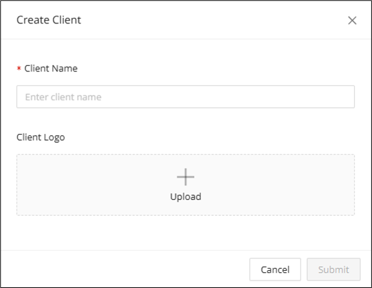
To display the actions available for this client, click the corresponding ... :
The following actions are available:
Edit client details
Select this action to display the client that you created earlier and edit the details that you entered there.
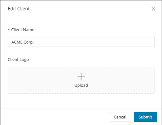
Edit client administrators
Use this action to create or remove client administrators. To create a new client administrator
-
In the Add Member field, enter the e-mail address of the new client.
-
Click Add .
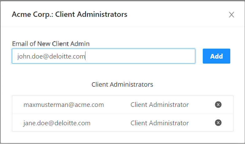
To remove a client administrator, click in the corresponding row.
Delete client and projects
To delete the client, check  Yes, delete Client including all projects and related data and click Delete .
Warning
Deletion of a client triggers a cascading delete on any artifacts belonging to the client. This includes projects, modules, taxonomies, sources, etc.
Managing projects
Info
Users with the role "Admin" can see all projects, users with the role "Client Admins" can see specific clients, and users with the roles "Manager", "Editor", or "Viewer" are restricted to assigned projects. Users can enter projects via the corresponding client page; however, to do so, they must have the required role-based user access. For more details on who can view or perform which actions, refer to the sections Identity and Access Management (IAM) and the Access Matrix.
The Client and Project Management view allows administrators or client administrators to manage projects associated with a client in the Mining UI. In this view, admins or client admins can:
- List all available projects
- Add a new project
- Update a project's general information
- Create new project members and assign project roles
- Delete a project
After the project exists, return to Code Discovery and link the Eclipse project through Properties > mining. Discover Code cannot target the correct Mining project until this linkage is in place.
The actions are described in the following:
Add project
-
Enter a project title.
-
Select the client from the drop-down list.
-
Click Submit to complete the action.
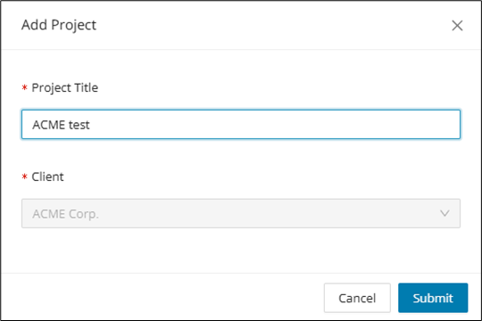
Edit project details
Select this action to display the Add Project window and edit the details that you entered there, for example, the project's title.
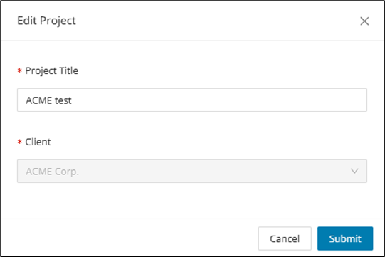
Edit members
Use this action to create new project members or to remove them. To do so,
-
In the Add Member field, enter the e-mail address of the new member
-
Select Viewer, Editor, or Manager as the project role.
-
Click Add to complete the action.
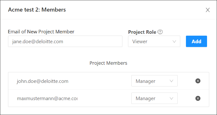
To remove a member, click in the corresponding row.
Delete project
To delete a project, check the box "Yes, delete Project including all related data," and click Delete .
Warning
Deletion of a project triggers a cascading delete on any artifacts belonging to the project. This includes projects, modules, taxonomies, sources, etc.
Additional web UI features
To learn more about additional Mining web UI features and functions, continue with the linked page. It covers supporting capabilities that complement the main reporting and analysis workflows. Use it when you want details on job handling, saved searches, error display, and related UI functions.
Click here.
Dashboard
After logging into the Mining Web UI and selecting a Client and Project, you will be led to the Dashboard page by default. The Dashboard is the default view of the Mining Web UI, and it provides spotlight overviews from the Code Discovery, including the number of missing source files and modules containing parser errors. Also, when conducting product demos, you can configure the "Showcase" mode on the View tab of the Configuration page, which will disable the display and red highlighting of parser errors on the Modules tile at the top of the page.
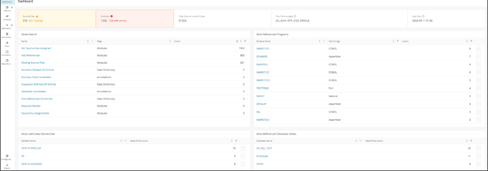
The Dashboard features a panel on the top, listing the number of Modules and Total Source Lines of Code, the Top Technologies, and the Last Scan date for Discover Metrics.
Additionally, information cards for the following categories are displayed:
| Category | Available Filters | Data Provided By |
|---|---|---|
| All Business Taxonomies | --- | Taxonomies, Identify Technical Taxonomies |
| All Taxonomies | --- | Taxonomies, Identify Technical Taxonomies |
| Saved Search | Name, Count | Discover Metric, Identify Candidates, Annotation |
| Most Referenced Programs | Module Name, Language, Value | Discover Metrics |
| COBOL Programs with Most File Descriptors (File In/Out) | Module Name, Language, Type, Value | Discover Metrics and Calculate Control Flow |
| Most Used Data Element/Set | DataSet Name, Read Write Count | Discover Metrics |
| Programs with Most Candidate Business Rules | Module Name, Language, Type, Value | Identify Candidates |
| Most Referenced Database Tables | Database Name, Read Write Count | Discover Metrics |
| Most referenced IMS Databases | Database Name, Read Write Count | Discover Metrics |
Info
If no data is available for the respective card, for example, if Discover Metrics has not been executed, the related cards above will be hidden from view.
Metrics
The visualization of metrics created by Code Discovery is central for the communication of the analyses and revealing unknown aspects of your codebase and data. A variety of charts and drill-downs is provided via the Metrics menu and its sub-pages. Most of these charts are interactive and will provide an overlay listing all related artifacts when they are clicked.
For example, in the Technologies page, clicking a blank area in a bar chart will list all related artifacts within the bar chart, while clicking a specific bar will produce a list of that bar only.
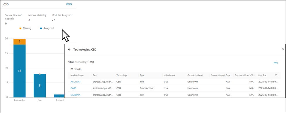
The following sections outline the various metrics available in the Mining Web UI.
Summary
The Summary page gives a quick overview of the number of Modules, files, lines of code, comments, dead code, missing modules, errors, and cyclomatic complexity by technology in tabular form. It is the fastest way to confirm overall project size, quality indicators, and discovery coverage in one place. Use it as a starting point before drilling down into the more specialized metrics pages.
Info
The table in the Summary page cannot be exported to CSV, but can be exported from the Export page by clicking "Download Effort Summary Excel".
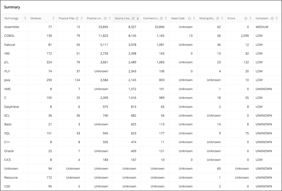
Technologies
The Technologies page displays a bar chart for each language discovered in the project. Each chart offers information about the lines of code and the number of missing and analyzed artifacts by module type. Hovering over a specific bar gives detailed insight into the missing and analyzed artifacts.
Info
Supported languages are Assembler, BASIC, C, C#, C++, CICS, Cobol, CSD, Easytrieve, ECL, IMS, Java, JCL, Natural, Oracle, PL1, Resource, SQL, and VMS. All others are listed as Unknown.
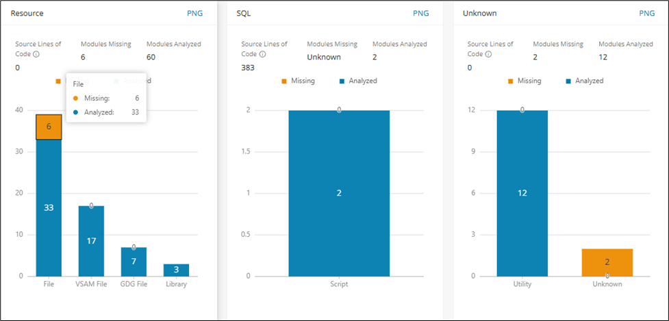
The displayed charts can be filtered by one or more taxonomies from the Filter by Taxonomy field at the top of the page.
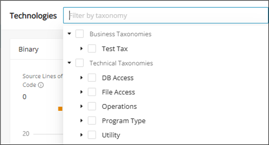
Utilities
The Utilities page delivers metrics about the project's utilities based on the categories they're invoked in. This view helps you see where shared utilities are concentrated across the portfolio. Use it to spot common helper components and the contexts in which they are invoked.
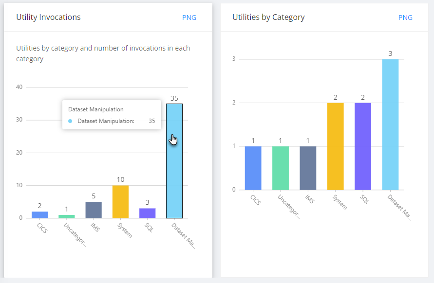
Interfaces
The Interfaces page shows utilities based on the interface type and the number of in- and outbound calls in each interface. This helps you understand how interface-related utilities are distributed across the codebase. Use it to compare inbound and outbound interaction patterns before investigating individual modules.
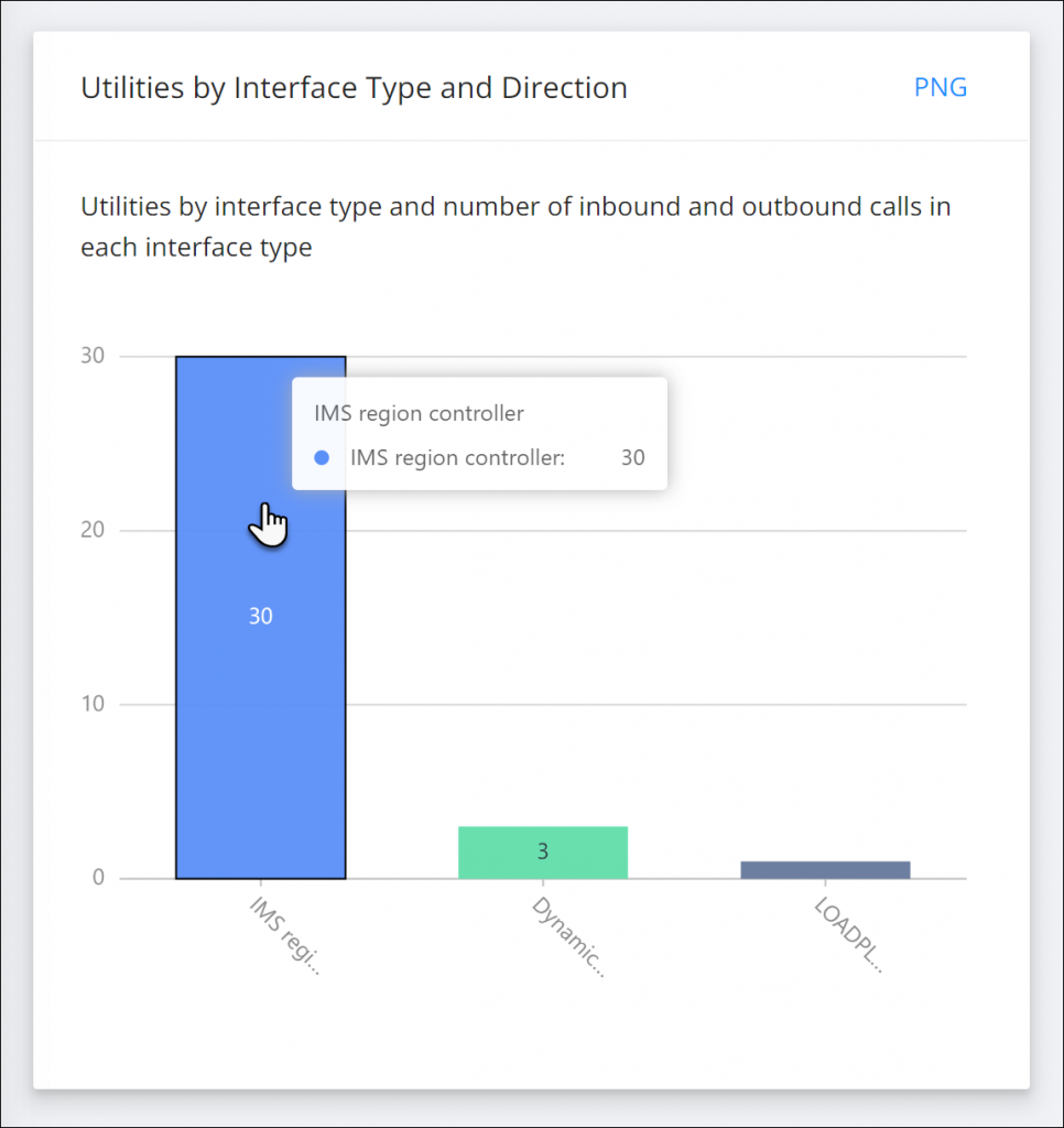
SQL
The SQL page offers charts analyzing the project's SQL statements. This view helps you assess how extensively SQL is used across the project. Use it to inspect statement-heavy areas and then open the related overlays for module-level detail.
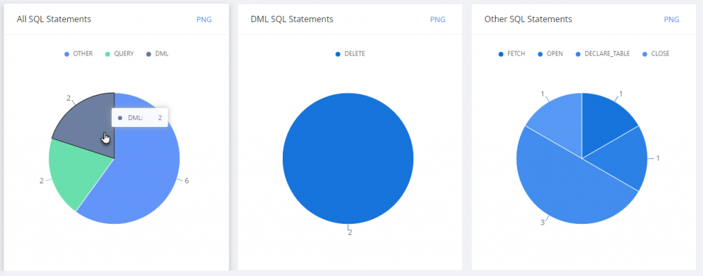
The displayed charts can be filtered by one or more taxonomies via the Filter by Taxonomy field at the top of the page.
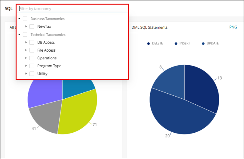
Clicking any of these charts will display a pop-up window with a table related to the chart. This table contains detailed information like the Module Name, Complexity, Technology, Type, etc. It is possible to click the module name to navigate directly to the module details page.
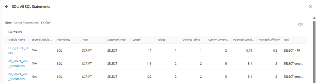
IMS
The IMS page offers charts analyzing the project's IMS calls and functions.
The displayed charts can be filtered by one or more taxonomies via the Filter by Taxonomy field at the top of the page.
In this view, it is possible to click the module name to navigate directly to the module details page.
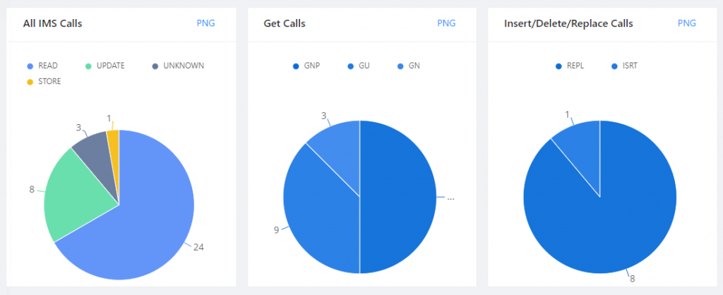
The following calls are supported:
| Function | Category | Description |
|---|---|---|
| GU | Get | Get Unique - like read |
| GN | Get | Get Next - like read next |
| GHU | Get | Get Hold Unique - specifies that a lock (hold) on the record happens after the unique record retrieval |
| GHNP | Get | Get Hold Next within Parent - get next within parent call, and locks (holds) the record |
| GHN | Get | Get Hold Next - reads the next record on the hierarchical data path and locks (holds) it |
| ISRT | Insert | Insert - adds new segments |
| DLT | Delete | Delete - removes segments |
| REPL | Replace | Replace - replaces segments used along with GHNP, GHU, or GHN |
| PCB | PCB | CICS programs |
| CHKP | Others | Checkpoint function - recovery process |
| XRST | Others | Restart function |
IDMS
IDMS is a network-style mainframe database platform used by many long-running enterprise systems. In a typical estate, business logic lives in COBOL and PL/I programs that issue IDMS DML (Data Manipulation Language) statements and navigate schema structures such as records, sets, areas, and subschemas. Modernizing IDMS is rarely a matter of syntax conversion alone. The harder problem is understanding the hidden behavior of the code: which programs read versus update which records, how set relationships drive data navigation, and where control flow and data dependencies create migration risk.
The IDMS page brings this intelligence together in a dedicated metrics area aligned with modernization planning. Code Discovery parses IDMS usage across COBOL and PL/I to build the inventory, dependency, and distribution views described below. Use the sub-menu on the left of the page to move between the Summary, DML operations, DML statements, Program record dependency, Language distribution, and IDMS schema structure views.
Key IDMS terms
These terms appear throughout the IDMS views:
- Schema: the full IDMS database definition, covering all record types, sets, and areas.
- Subschema: a program-specific view of a schema that exposes only the records, sets, and areas a program needs.
- Record: a business data object, such as customer or order data.
- Set: an owner-member relationship that links records and drives navigation between them.
- Area: the storage zone where related records are physically organized.
- DML (Data Manipulation Language): the statements programs use to read and change the database, such as
OBTAIN,FIND,STORE,MODIFY,ERASE,CONNECT, andDISCONNECT. - Currency: the pointers that track a program's current position in the database during DML execution, spanning run-unit, record, set, and area currency.
- DB, DC, and LRF: DB statements access stored database records, DC (data communication) statements handle online and terminal interaction, and LRF (Logical Record Facility) statements access data through logical records that can span several physical records and sets.
Summary
The Summary page is the landing view for IDMS and gives a high-level snapshot of the IDMS footprint. The header cards report the Total programs, Total lines of code, and DML statements discovered. The Program language breakdown chart shows the split between COBOL and PL/I, while the IDMS entities and Architecture components panels count the schema building blocks (total entities, sets, areas, maps, schemas, and subschemas) alongside the lines of code contributed by each language. The Top schema by size chart ranks schemas by the number of components they contain.
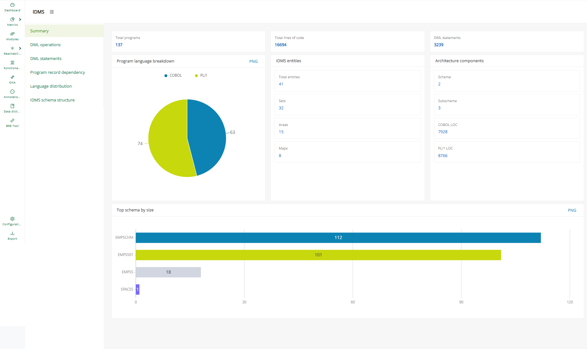
Use this page to confirm the overall size and composition of the IDMS estate before drilling into the more specialized views.
DML operations
The DML operations page describes how the code interacts with the database at the operation level. The DML by category chart groups statements into retrieval, modification, control, accept, DC terminal, and LRF categories to reveal the dominant access patterns. The DB vs DC split chart separates database (DB) access from data communication (DC) activity, and the Top 10 DML verbs chart ranks the most frequently used verbs, such as OBTAIN, BIND, FIND, and FINISH.
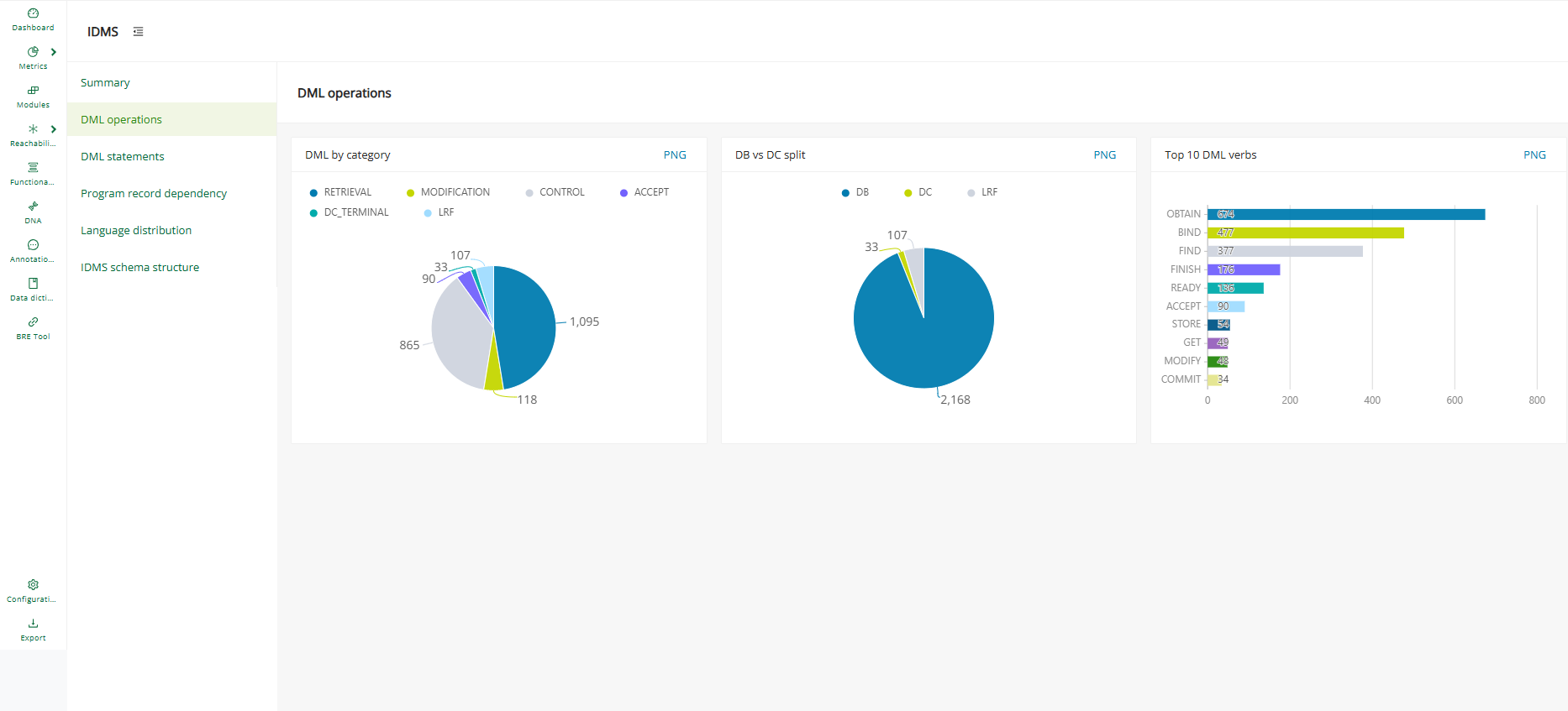
DML statements
The DML statements page quantifies IDMS statements in more detail. The DML category distribution card summarizes the total statements split across DB, DC, and LRF, and separate cards break the totals down into Retrieval calls, Modification calls, Recovery statements, Accept statements, and the DC Category. Each card lists the verbs that make up its category, so it is easy to see which retrieval, modification, or recovery verbs dominate the codebase.
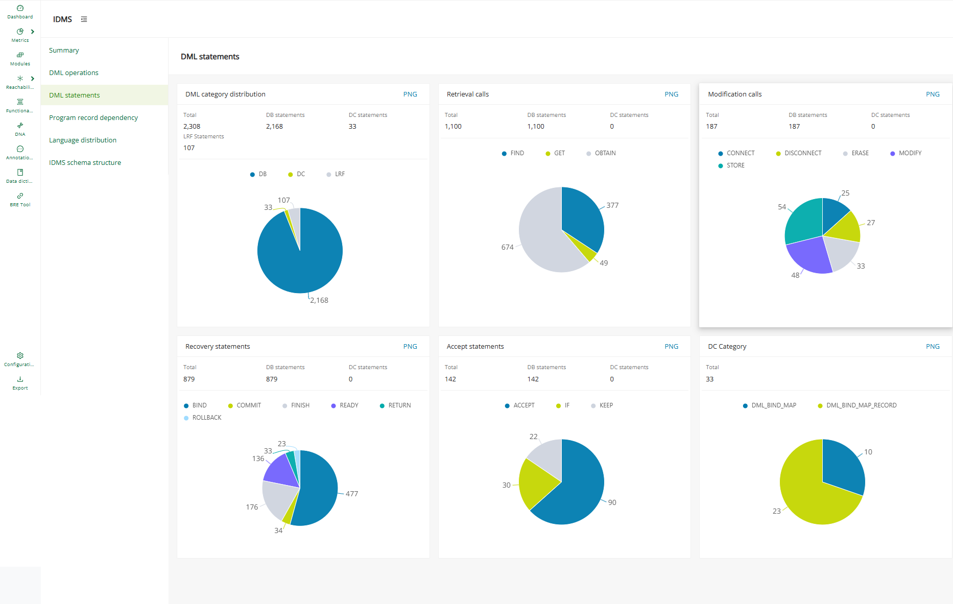
Program record dependency
The Program record dependency page lists the programs that interact with IDMS records and sets, supporting impact and change analysis.
Select a program name to open its dependency diagram that shows the Record and IDMS set nodes the program touches and the OWNER and MEMBER relationships that connect them. Use the zoom, fullscreen, and Show orphan nodes controls to explore the diagram, and the About this graph button for the legend and guidance.
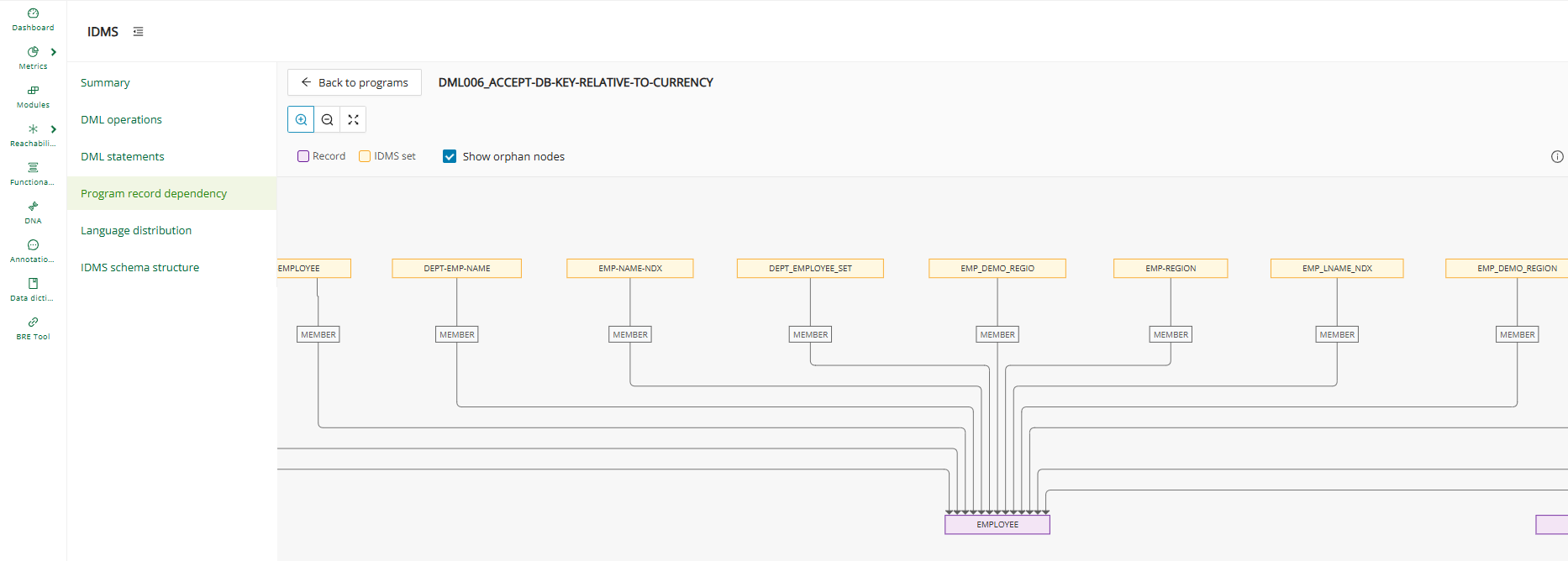
This view answers core change-impact questions early: if a record or set changes, which programs are affected, and which areas of the estate are tightly coupled.
Language distribution
The Language distribution page shows where IDMS logic resides by language (COBOL versus PL/I) to help sequence migration work. Narrow the chart to a subset of the codebase with the Filter by taxonomy field at the top of the page.
IDMS schema structure
The IDMS schema structure page presents schema-level components and their relationships to support architecture understanding of the IDMS database design.
Decomposition
The Decomposition page shows metrics for Technical Taxonomies according to the category they were assigned to in the project, for example, (batch vs online).
The displayed charts can be filtered by one or more taxonomies via the Filter by Taxonomy field at the top of the page.
The overlay contains a table with additional information like the module name, the path to the module, the technology, and the lines of code. It is possible to click the module name to directly get to the module details page.
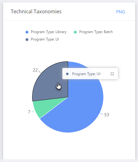
Info
As a prerequisite, the Identify Technical Taxonomies feature needs to be executed from the Modules Reporting page to gather the corresponding data.
Code quality
The Code Quality page hosts various charts about the project's complexity, code lines, job steps, and SQL statements.
The displayed charts can be filtered by one or more taxonomies via the Filter by Taxonomy field at the top of the page.
The overlay contains detailed information such as the kind of statement, the complexity, and the lines of code. Click on the zoom icon to have a closer look at any Code Quality chart.
Complexity analysis
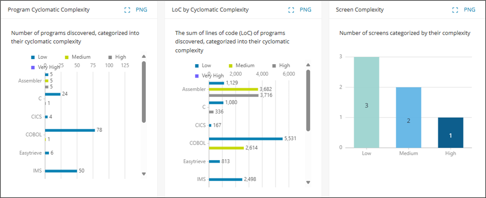
| Metrics | Definition |
|---|---|
| Cyclomatic Complexity | The complexity Level calculation uses the standard McCabe formula to apply a common definition of cyclomatic complexity for supported programs. It quantifies the number of independent linear paths of a program based on its control flow. The formula used to calculate the complexity score is as follows: C = N + 1 (where N is the number of decisions/conditions). |
Info
For Cyclomatic Complexity, the low-to-high program scoring categorization is applied based on the underlying complexity score: Low: 1-10, Medium: 11-20, High: 21-50, Very High: >51
Code lines analysis
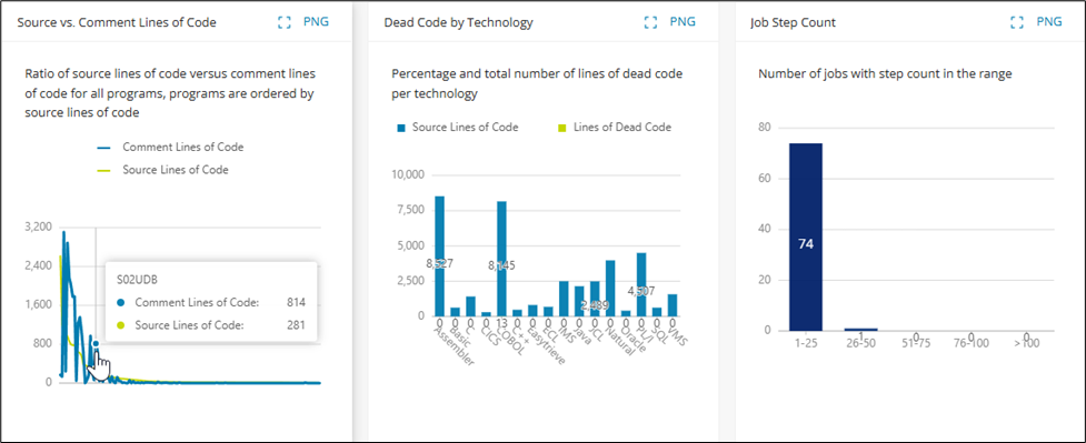
| Metrics | Definition |
|---|---|
| Source Lines of Code | The code line count of a module is the sum of non-blank lines in the unassembled source containing code instructions of that language. Comment lines do not count toward the source lines of code. |
| Comment Lines of Code | The comment line count of a module is the sum of non-blank lines in the unassembled source containing only a comment instruction of that language. Lines that contain code and comments do not count toward the lines of comments. |
| Dead Code | Dead code describes lines of code found to be unreferenced or unused, and therefore never executed at runtime. |
SQL analysis
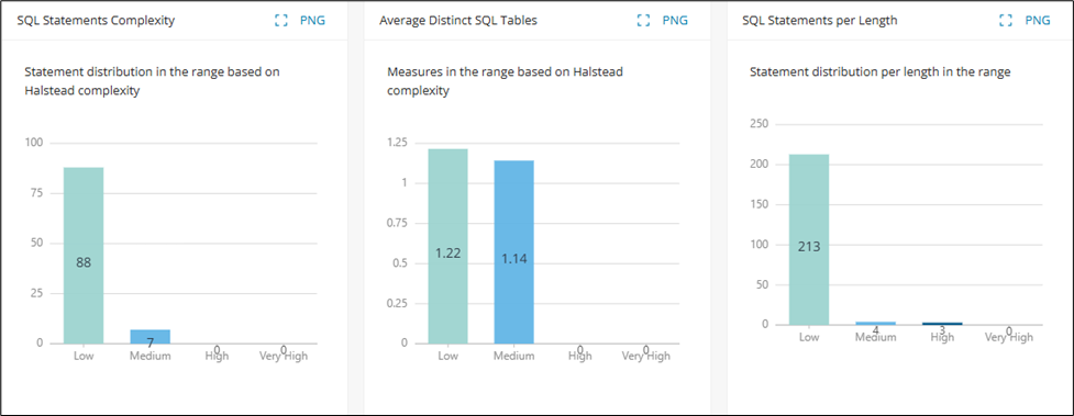
| Metrics | Definition |
|---|---|
| Statement Complexity | Represents the complexity of an SQL statement based on the overall amount of parsed SQL nodes, for example, (Operators, Identifiers, Literals) that comprise the statement. |
| Halstead Complexity | The Halstead complexity calculation measures the complexity of a program by looking at the number of operators and operands and their overall usage. Halstead complexity scoring categories are applied based on the underlying complexity score and statement length: - Low: 1-10 (1-400 characters) - Medium: 11-20 (401-800 characters) - High: 21-50 (801-1200 characters) - Very High: >50 (>1200 characters) |
| Distinct Tables | Distinct tables are all tables accessed by modules, not accounting for duplicates/repeated access of the same table. |
Candidates
The Candidates page visualizes the data gathered as a result of executing Identify Candidates.
The displayed charts can be filtered by one or more taxonomies via the Filter by Taxonomy field at the top of the page.
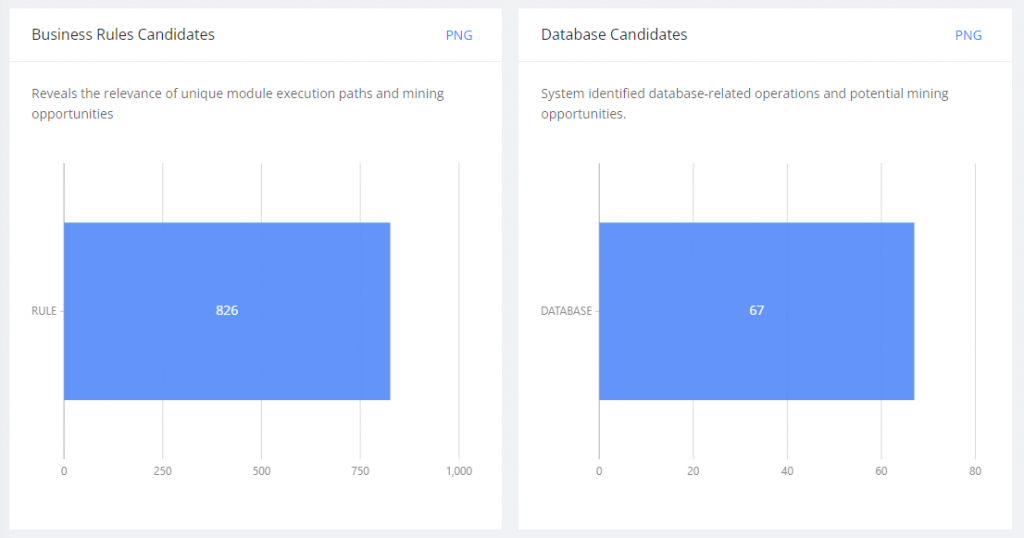
Info
As a prerequisite, the Identify Candidates feature needs to be executed to gather the corresponding data.
Modules
Modules
Modules are generated during Discover Metrics (code base upload) to encapsulate discovered system artifacts, for example, source files, SQL scripts, etc., from the code base, along with any generated metadata such as annotations, dependencies, metrics, taxonomies, data dictionary entries, and descriptions, providing increased context on those system artifacts. Changes to Modules are updated from incremental Discover Metrics scans and will be reflected in the Mining Web UI.
To open a list of all available modules, select Modules from the categories on the left. The page displays all discovered modules with their name, technology, type, and the last scan date for Discover Metrics. The number of results is displayed above the modules table, along with a button to export the table information in CSV format.
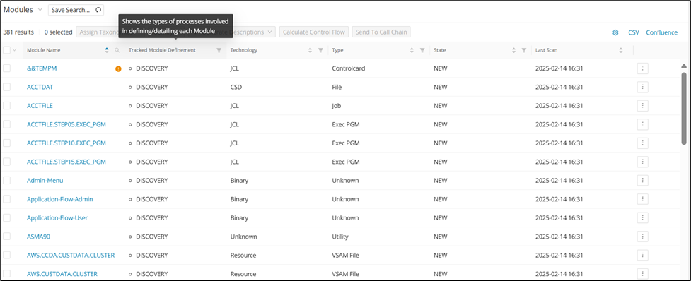
Info
The Modules menu item, as well as each affected module in the table, will be marked with an orange badge if they require review. Modules are marked for review if they contain metadata (for example, annotations, taxonomies, data dictionary entries, module descriptions) and changes to the module code are detected after incremental Discover Metrics scans.
Using the modules table
To narrow down results, you can search by Module Name. To do so, click the search icon in the Module Name column and enter a partial or full Module name, then click Search . To reset the search and display the full list of modules, click the search icon again and click Reset .

To filter columns, for example, by Technology or Type, click the corresponding filter icon and select the appropriate entries from the drop-down lists. You can select multiple values for each filter.
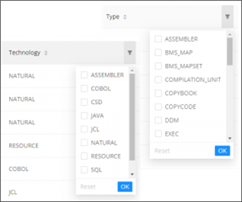
To directly access a module in Code Viewer or open its Control Flow or Dependency Graph, select the corresponding link in the shortcut menu, designated by the three dots on the rightmost column.
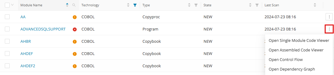
It is also possible to filter columns with the filter option "None" to get a result in which entities (modules, annotations, data dictionary) don't have a value assigned to a certain data point.
Once the desired modules are displayed, you can export the list by clicking CSV in the top right corner.
Feature overview
The Modules area combines bulk toolbar actions with module-level investigation and editing workflows. Use the following overview to jump directly to the corresponding feature page.
| Feature | Description |
|---|---|
| Assign Taxonomies | Assign technical and business taxonomies from the modules table, including Taxonomy Propagation to extend selected taxonomy assignments across related dependencies. |
| Identify | Run bulk identification workflows from the modules table, including candidate identification, dead-code analysis, technical taxonomy assignment, module descriptions, functional blocks, and process sequencing. |
| Generate Descriptions | Generate GenAI-assisted annotation, module, and Data Dictionary descriptions from the modules table, with options to add context and improve output quality. |
| Calculate Control Flow | Pre-calculate control flow graphs for selected modules so the Control Flow Graph loads faster later from Module Details. |
| Calculate Data Lineage | Pre-calculate data lineage for selected modules and fields so lineage views open faster when needed. |
| Send to Call Chain | Send selected modules directly to the Call Chain workflow so you can visualize inbound and outbound connectivity without rebuilding the selection manually. |
| Code Viewer | Investigate individual modules in detail, review metadata and relationships, and perform module-level editing workflows from the code-centric analysis view. |
| Module Details | Open the detailed module page to review metadata, metrics, dependencies, and generated artifacts tied to a specific module. |
Assign Taxonomies
Taxonomies are used to categorize and organize modules within a project and are categorized as either "Technical Taxonomies" or "Business Taxonomies" (configurable) to represent the technical categories of the application, for example, UI, Batch, etc., or the business domain of the application that each module belongs to. Modules can be assigned multiple taxonomies for maximum flexibility, including both Business and Technical Taxonomies. Business Taxonomies can be created and configured in the Configuration page.
When selecting modules in the modules table, there is an option to assign taxonomies directly from the Modules page.
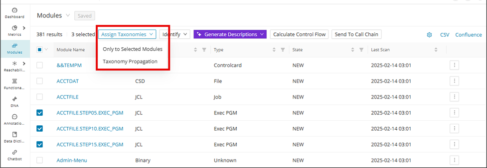
Select one or more modules and then click the Assign Taxonomies drop-down, and then click Only to Selected Modules . A window for assigning taxonomies will display on the right-hand side, in which you can check the taxonomies and assign them to the selected modules.
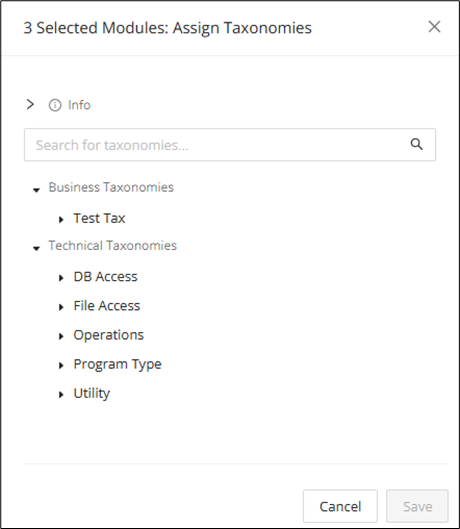
After assigning modules the appropriate Technical and Business Taxonomies, teams can gain a clearer picture of their system's structure and domain relationships from various outputs such as tables, graphs, and models. For example, when coupled with Social Graphs, teams are enabled with a visual that represents a high-level overview of the application's business domains, which supports informed modernization decision-making.
Info
Social Graphs are currently built using third-party tools (for example, Gephi) and are not built into Mining at this time.
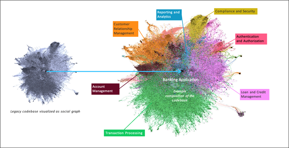
Taxonomy Propagation
Taxonomy assignment is a mostly manual and labor-intensive task, especially when users must individually assign taxonomy terms to every module or use Taxonomy Batch Import. Taxonomy Propagation streamlines the process of assigning taxonomies to modules by automatically propagating taxonomies from parent modules to their dependent child modules and vice versa. Simply assign taxonomy terms to starting modules, and the Code Discovery & Mining intelligently applies these categories throughout related dependencies.
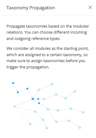
Navigate to the Modules page, select the module(s) to propagate, and click Taxonomy Propagation.

The Taxonomy Propagation window opens as a drawer on the Modules page, from which the user can select the taxonomies to propagate and select the outgoing reference(s).
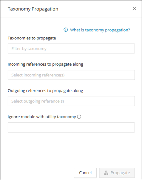
After making selections, click Propagate to open a window to see the modules that will be propagated. Click Proceed after confirmation. Note that taxonomy propagation cannot be reversed once applied and would have to be manually removed from the affected modules.
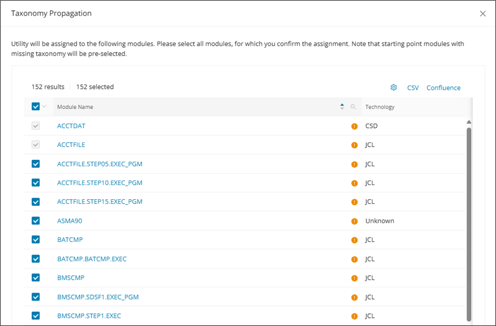
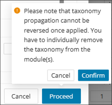
After Taxonomy Propagation is complete, click on the affected module(s) to access the Module Details and verify the taxonomies.
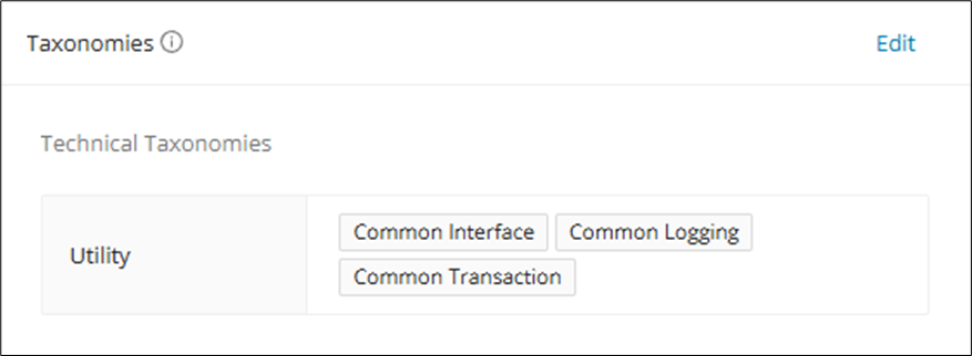
Propagation with conditional dependency
By default, Taxonomy Propagation logic uses module references and does not use call chains to identify dependencies between modules; thus, they also cannot account for conditional dependencies. To enable conditional dependency identification, enable the feature toggle callChainBasedTaxonomyPropagation, then run Taxonomy Propagation.
Configuration
The feature toggle callChainBasedTaxonomyPropagation has to be enabled for this feature.
Identify
When selecting modules in the modules table, there is an option to identify candidates, dead code, technical taxonomies, module descriptions, and functional blocks directly from the Modules page. Click the Identify drop-down above the modules table to open a menu with the following options. Use these actions when you want to generate candidate metadata or structural analysis without opening each module individually.
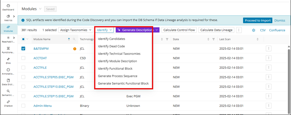
- Identify Candidates: Identify system rules, DB operations, and Data Dictionary Entries.
- Identify Dead Code: Identify dead code based on control flow and annotate the dead code.
- Identify Technical Taxonomies: Identify technical system domains and usages, for example, batch, UI, File read/write, etc., automatically assigning these technical taxonomies to supported modules.
- Identify Module Description: Provides an initial module description in the system based on the source code (comment-based). However, for a Gen AI-based module description (recommended), refer to Generate Module Descriptions.
- Identify Functional Block: Generates Functional Blocks for the selected modules based on the skeletal outline of the program, for example, (PGMNAME (Parent FB) -> PARA1 (Child FB) - PARA2 (Child FB) - PARA3 (Child FB)).
- Generate Process Sequence: Generate a process flow sequence of existing annotations on each module.
- Generate Semantic Functional Block: Generates Functional Blocks for the selected modules based on related functions within the program.
Info
To use Identify Candidates for Action and Condition Annotations, enable the feature toggle identifyActionConditionAnnotations.
Automated Annotation generation for Java
Single and bulk auto-annotation generation can be done, and the generated annotations will be related only to the Business rule. This option is intended for Java compilation units that you want to annotate quickly from the Modules table. The steps below show the basic selection and execution flow.
Select Technology as Java and Type as Compilation Unit.
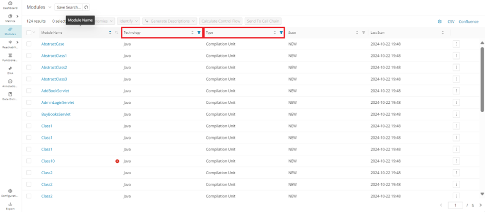
Select the modules and click Identify Candidates .
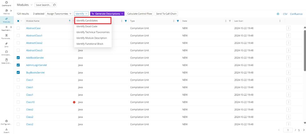
Annotation for category Business Rule is generated
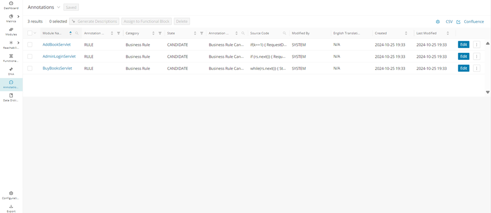
Generate Process Sequence for Annotations
After extracting Business Rules with Identify, you can run into the time-consuming, mistake-prone process of manually sequencing the generated annotated rules. "Generate Process Sequence" automates the sequencing of functional business logic, significantly reducing the time and effort required for manual processing.
From the Modules page, select the module(s) to automate the sequencing, click Identify , and then click Generate Process Sequence .
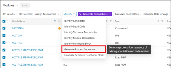
After the "Generate Process Sequence" job is complete, each annotation will have a new Process Sequence datapoint that is auto-populated.
Generate Semantic Functional Block using GenAI
Generate Semantic Functional Block uses GenAI to group related code into higher-level functional units. It is intended for cases where structural grouping alone does not capture the logical process flow. Review the generated results carefully, because the output is based on AI interpretation of the control flow.
Configuration
The feature toggle semanticFunctionalBlockGeneration must be enabled in the WebUI feature console.
A semantic functional block is similar to a functional block, but feeds its control flow graph to GenAI to generate the functional process flow. Semantic functional blocks find and group code snippets that may be related to one another to create a more comprehensive block. As with all GenAI-generated content, be sure to check for accuracy.
Click Identify and then click Generate Semantic Functional Block .
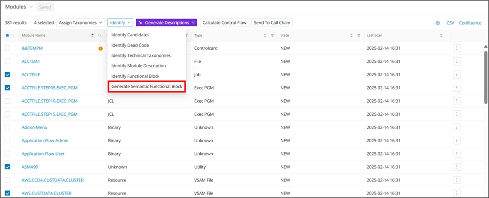
After clicking Generate Semantic Functional Block ,a pop-up window appears for configuration of the desired semantic functional block.
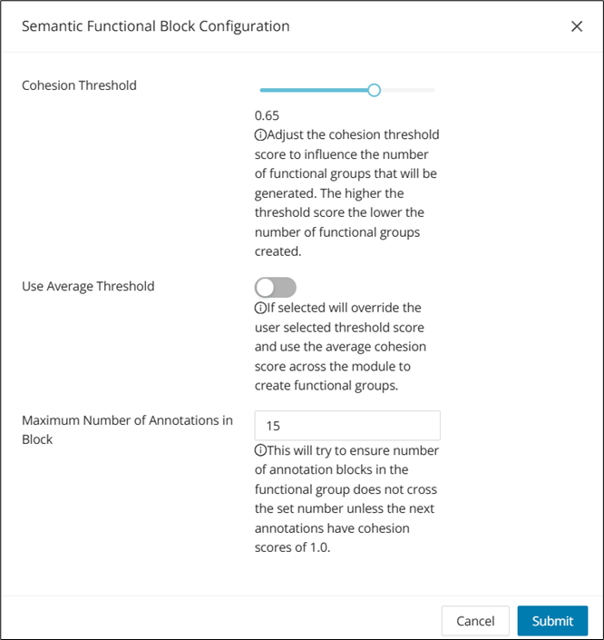
After choosing the desired configurations, click Submit to generate the semantic functional block.
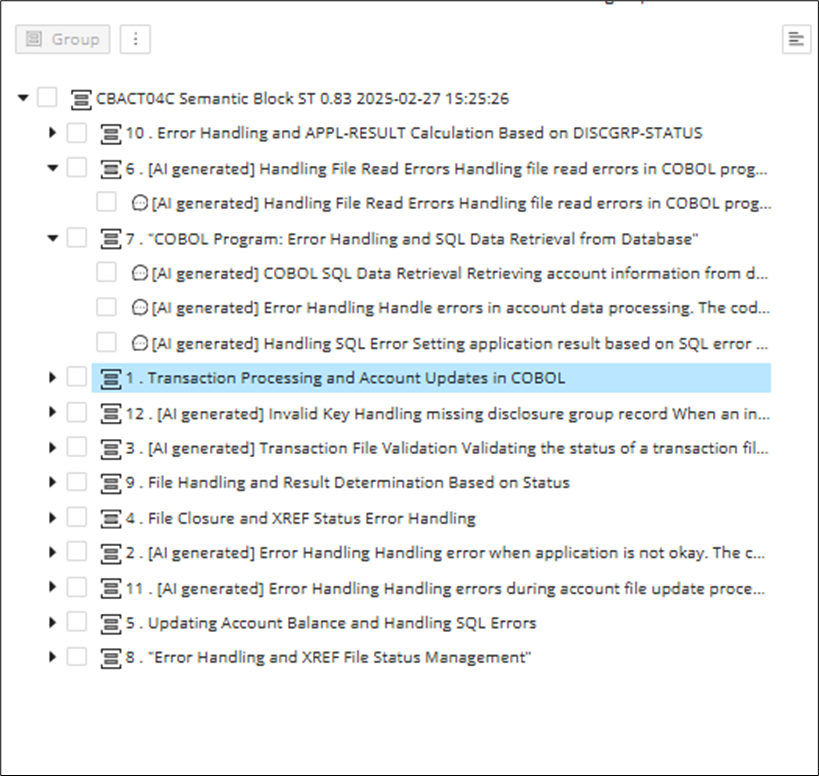
Generate Descriptions
Generate Descriptions lets you add AI-generated annotation, module, or Data Dictionary descriptions directly from the Modules page. It is useful when you want consistent first-draft text for a selected set of artifacts. Review the generated output before publishing or relying on it in analysis.
Configuration
The feature toggle generativeAiTranslations must be enabled in the WebUI feature console.
When selecting modules in the modules table, there is an option to add AI-generated annotation, module, or Data Dictionary descriptions from the Modules page. Click the Generate Descriptions drop-down above the modules table to open a menu with following options:
- Generate Annotation Descriptions
- Generate Module Descriptions
- Generate Data Dictionary Descriptions
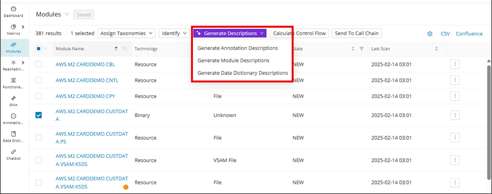
Generate Annotation Descriptions
Select the type of description (Annotation, Module, or Data Dictionary) that needs to be generated. In this example, we want to generate annotation descriptions, so click Generate Annotation Descriptions and then click Generate in the following confirmation window. If the selected modules already contain user-written descriptions, they can be overwritten by clicking the checkbox.
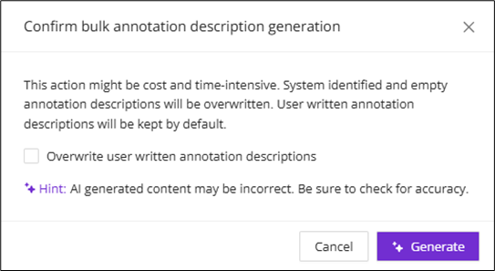
To view the newly generated annotations, click one of the selected modules to enter its Module Details page and click the "Annotations" tab.
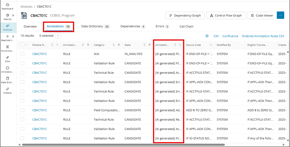
Annotations can also be automatically generated directly from the Annotations page as described in Bulk Generation of Annotation Description.
Advanced AI options
To increase the accuracy of generated annotation descriptions, you may want to consider providing further context from the Advanced AI Options feature. First, access the edit pop-up on the annotation for which you want to generate a more accurate description (you can access this edit from Module Details, Code Viewer, or the Annotations page). From here, click the settings icon next to Generate to open Advanced AI Options.
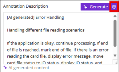
Provide context (for example, meaning of variables, purpose of system, etc) to the annotation that you want the GenAI to capture in the description, and then click Add Context.
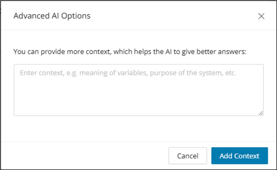
Generate Module Descriptions
Configuration
There is an option to generate module descriptions based on functional blocks. Enable the structuralFunctionalGroups feature toggle to access this feature.
First, select the modules that need to generate descriptions and then click Generate Module Descriptions from the drop-down list. With the structuralFunctionalGroups feature enabled, a new checkbox for generating module descriptions based on functional blocks will be displayed. Check this box and click Generate .
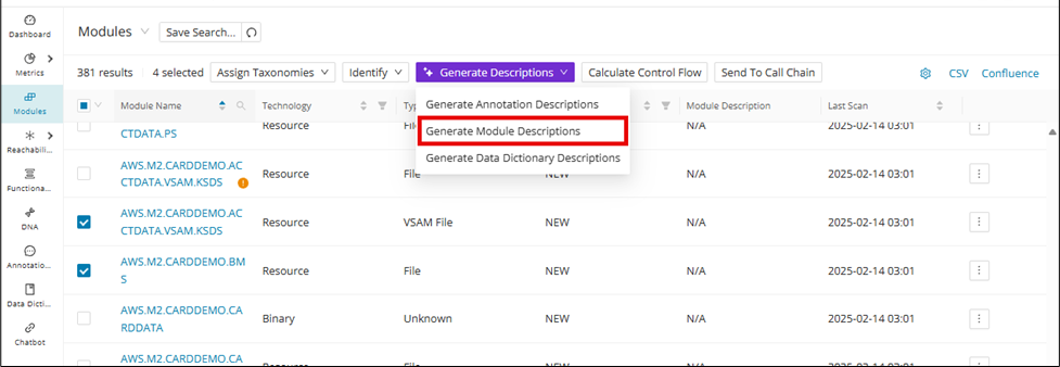
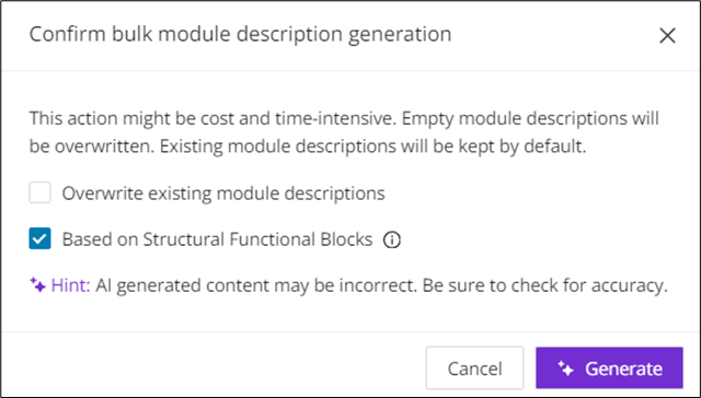
The module descriptions associated with the selected modules will be updated under the "Module Description" column.
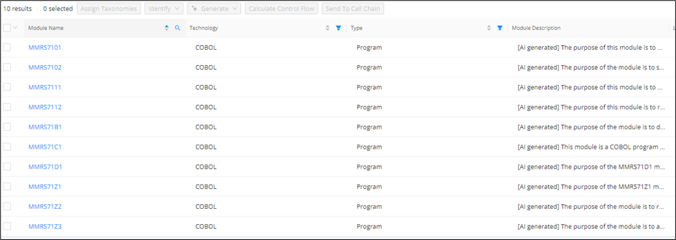
Generate Data Dictionary Descriptions
Info
Data Dictionary Entries must already exist for selected modules before generating their descriptions. Running Identify Candidates on supported modules will auto-generate the Data Dictionary Entries for application fields, for example, (variables, CICS, file record layout), while uploading a DB Schema or executing Discover Metrics on a project containing SQL DDL Scripts will create the SQL-related entries.
To generate Data Dictionary Descriptions, first select the module(s) for generation and click Generate Data Dictionary Descriptions from the drop-down menu. Click Generate in the following confirmation window.
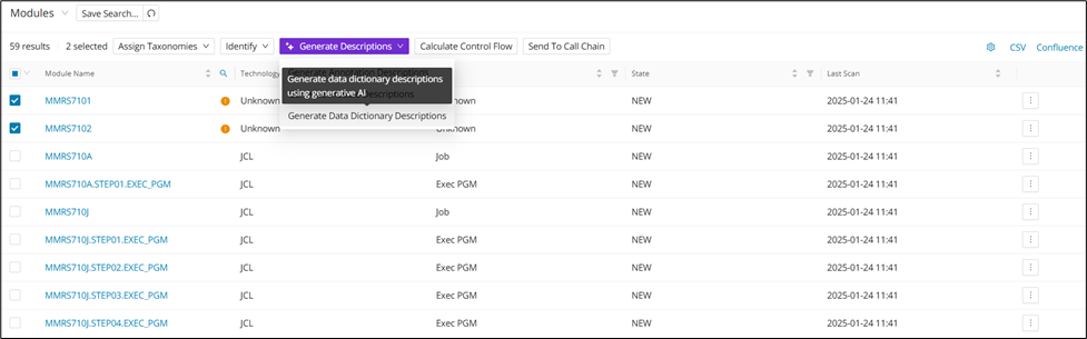
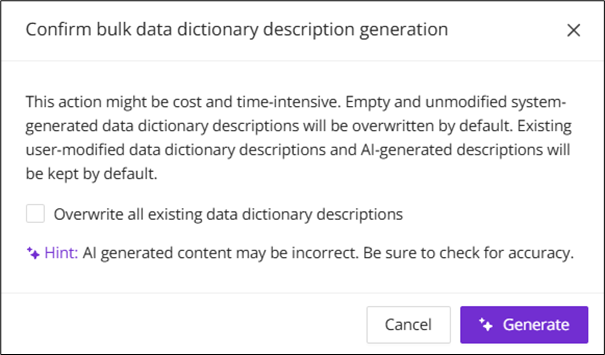
To find the newly generated descriptions, click on one of the selected modules to open up its Module Details page, then click the "Data Dictionary" tab.
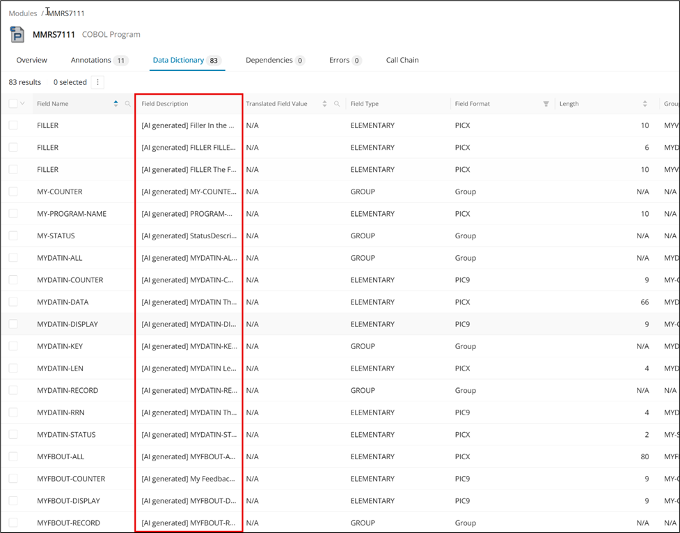
Data Dictionary descriptions can also be automatically generated directly from the Data Dictionary page, as described in Bulk Generation of Data Dictionary Description.
Calculate Control Flow
When selecting modules in the Modules table, there is an option to trigger the Calculate Control Flow job directly from the Modules page. This job refreshes the control flow data that other Mining views rely on. Use it before opening diagrams when you want the latest control flow information available.
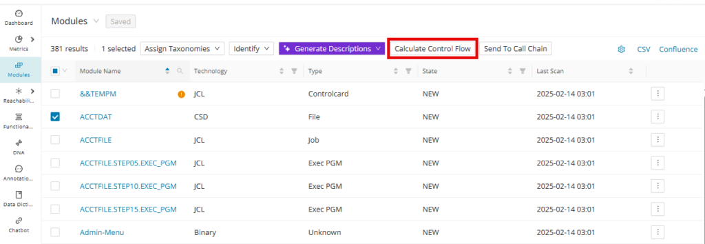
Click Calculate Control Flow to recalculate the control flow graph for the selected modules. This allows faster loading of ASTs once the control flow diagram is opened from the corresponding Module Details page.
Calculate Data Lineage
Generating data lineage graphs can be a process-intensive operation depending on the data flow path of the application. Similar to Calculate Control Flow, pre-calculating the data lineages of the selected fields and module(s) and then storing the results will shorten the wait time it otherwise could have taken to Show Data Lineage.
Select the module(s) for pre-calculation and click Calculate Data Lineage .
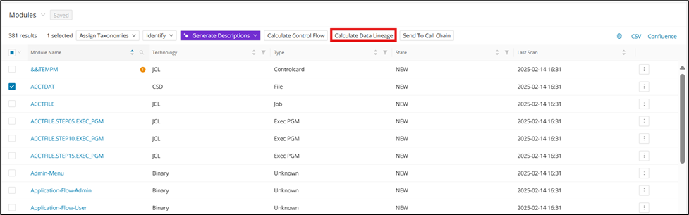
The pre-calculated module(s) will have their data lineages ready to view.
Send to Call Chain
Click Send to Call Chain to send selected modules from the Modules page to the call chain. This shortcut preserves your current module selection and opens it in the call chain workflow. Use it when you want to move from module reporting directly into dependency path analysis.
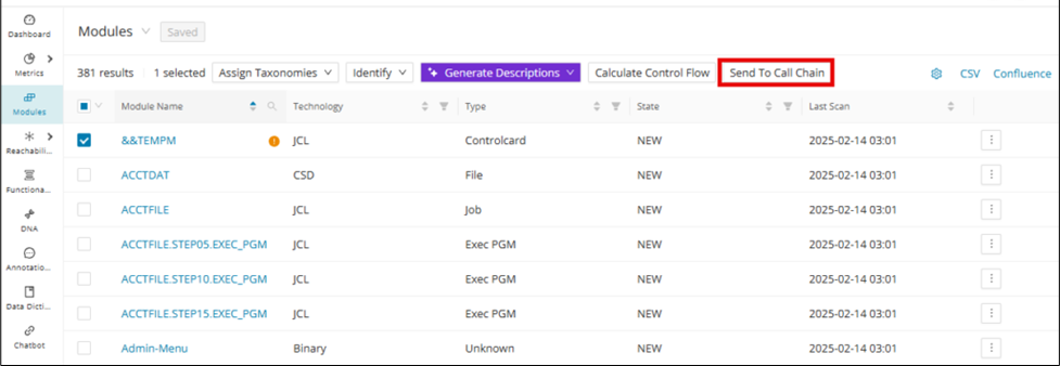
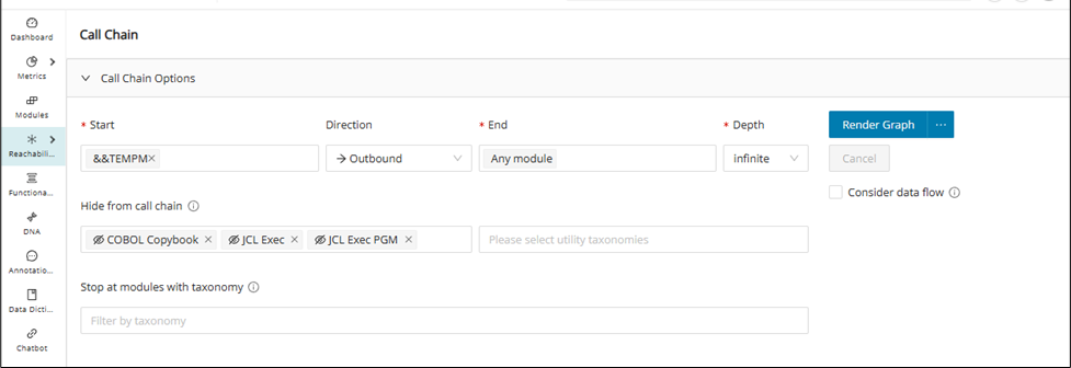
Code Viewer
The Code Viewer in the Web UI enables you not only to view annotations and data dictionary entries, but also to perform actions similar to those in Eclipse. To view the code, go to the Modules page and select the desired module. Then click Open Single Module Code Viewer to view the unassembled source and click Open Assembled Code Viewer to view the assembled source.
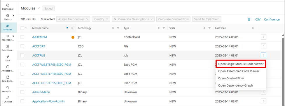
From here, you can view the read-only code of the selected module, from which you can either:
- Open Assembled/Single Module View
- Create/Edit Annotations
- Create/Edit Data Dictionary Entries
- Navigate Source via Hyperlinking
- Filter Annotations, Data Dictionary Entries, and Hyperlinking
Code Viewer assembled view
The Code Viewer provides an assembled view for languages (for example, Cobol, Natural, JCL, and PL/1) that use assembling. This view combines the root source with included artifacts so you can inspect the effective code in one place. Use it when copybooks or similar includes make the single-module source incomplete.
Info
COBOL, Natural, JCL, and PL/1 are supported.
Configuration
For this view, the feature toggle codeViewerAssembledView must be enabled in the WebUI feature console.
To access the assembled view from the Code Viewer, click Open Assembled View displayed at the top of the page.
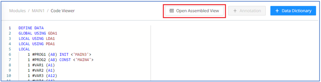
This opens a new tab with the assembled view. It contains the contents of all the included copybooks:
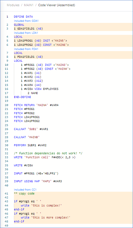
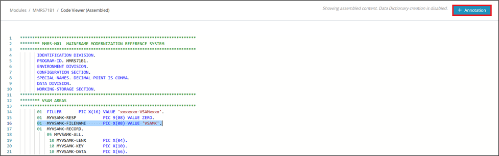
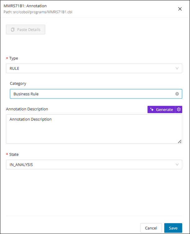

Annotating lines of source code spanning across the root program and included Copybook is not allowed.
+ Annotation is disabled.
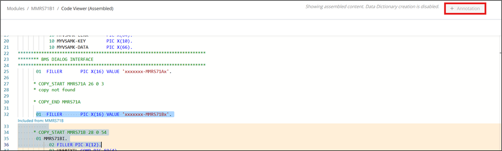
A tooltip is displayed while hovering above that "Annotating lines of code is not allowed across the root program and included Copybook".
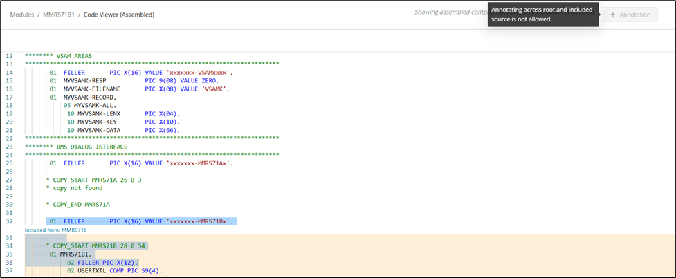
An annotation can be deleted from the CodeViewer (Single Module & Assembled view) by clicking the delete icon on the associated annotation summary bar.


Filter annotations and Data Dictionary entries by clicking the filter icon in the top right corner.
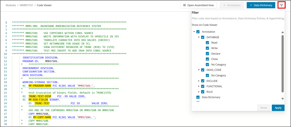
JCL symbolic parameter values
The assembled view for JCL can also resolve symbolic parameter values while you inspect a job. This helps you understand the effective runtime values without leaving the viewer. The note below describes how the hover behavior works.
Info
JCL only: Hovering over Symbolic Variables in the Assembled Code Viewer will show the actual value as a pop-up.

Annotations
With the Code Viewer, you can view, add, edit, and remove annotations. This makes the source panel a direct workspace for documenting code behavior while you review it. The following sections describe the main creation and management actions.
Creating an Annotation in Code Viewer
Step 1:
Mark the section of code for which you want to create an annotation, then click + Annotation on the upper right. Alternatively, mark and right-click the section of code, then select Create New Annotation from the context menu.
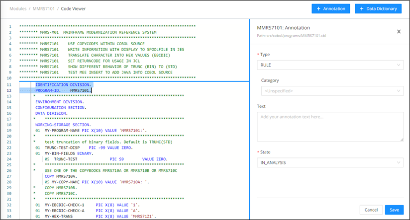
Step 2:
When the annotation editor opens, complete the fields below:
- Type: Select the type of annotation from the dropdown list. The following types are available:
- Database
- Dead code
- Exclude
- Rule
- Category: Select the category (Optional).
- Text: Add a suitable description of the selected code in the text box.
- State: Select the appropriate state from the dropdown list. The following states are available:
- Candidate
- In Analysis
- For Review
- Rejected
- Approved
- Invalid
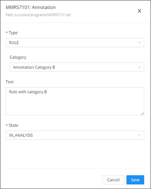
Step 3:
Click Save to complete the annotation.
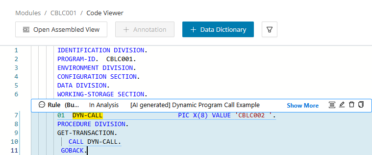
Annotation description with Gen AI
Generate allows users to generate an AI-based annotation translation for the created annotation. The generated description might change with each use of this feature.
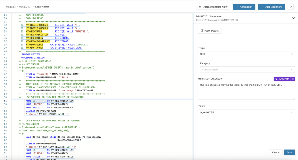
Configuration
The feature toggle generativeAiTranslation must be enabled in the WebUI feature console.
Managing Annotations in Code Viewer
After you create an annotation, it will appear directly in the Code Viewer. You can also locate the same annotation in the Annotations page for additional details (see Annotations). From the Code Viewer, you can manually manage each annotation using the actions described below.
Functional Blocks group one or more annotations into a higher-level "block of functionality," so you can describe code behavior at a process level. From the Code Viewer, click on the Functional Block icon to create Functional Blocks and assign them to annotations. For other creation options, see Functional Blocks Creation
Functional Block Modal from Code Viewer
In Code Viewer, on the annotation overlay, click the Functional Block icon to open the "Assign Annotation to Functional Block(s) modal.
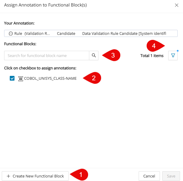
1. + Create New Functional Block : Click to create a new functional block.
Create New Functional Block Walkthrough
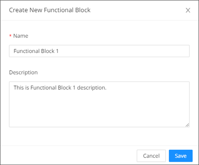
Enter the Name and Description and then click Save . The annotation will automatically be assigned to the newly created block.
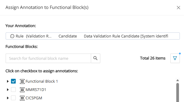
Warning
Duplicate Functional Block names aren't allowed within the same module.
2. Assign/Unassign Checkboxes: Check to assign the annotation to a Functional Block; uncheck to unassign.
3. Search: Search Functional Blocks by name/keyword to quickly locate the right one.
4. Filter: Narrow the list of Functional Blocks to your liking from the filter modal.
Functional Block Filter Walkthrough
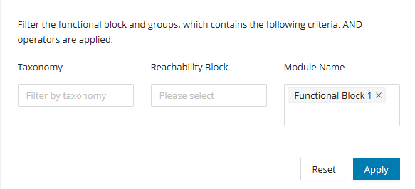
Enter the taxonomy, reachability block and/or module name to filter and click Apply . To reset the filter click Reset .
Click the Edit icon in Code Viewer to open the Annotation Edit side panel, where you can review and update the annotation's details (copy/paste annotation, type and category, English translation, description generation, and state).
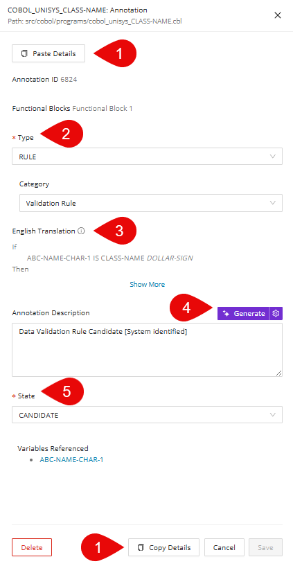
1. Copy/Paste Details: Click Copy Details to copy an annotation's full set of fields, then open another annotation and click Paste Details to apply the same values and make it identical. See Annotation Copying and Pasting for more annotation copy/paste options.
Copy/Paste Details Walkthrough
Here is an example of two annotations that contain different fields. Follow these steps to make them identical.
First, click the edit icon of the annotation you want copied and click Copy Details . The button will change to Copied to indicate the annotation's details are ready to be pasted. Then open the annotation you want the details to be pasted to and click Paste Details .
2. Type & Category: Use Type & Category to place annotations into main categories (Type) and further classification (Category) if needed. See Annotation Types and Categories for more information on each Type and Category. You can also add custom categories under the Configuration page (see Annotation Configuration)
3. English Translation: Shows a plain-English rendering of the annotation logic to make the code intent easier to review and validate (see English Translation Data point).
4. Generate Annotation Description: Click Generate to auto-draft the annotation description using GenAI, or click the Advanced setting icon to open the Advanced AI Options modal and fine-tune how the description is generated. See Generate Annotation Descriptions for more context.
5. State: Sets the annotation's current lifecycle status to support review, filtering, and workflow.
Click the delete icon. You will be given a confirmation dialog before completing the action. Click Delete to finalize your decision.
Click the Copy icon to save the annotation details from the Code Viewer. Find (or create) a target annotation, then click Paste Details to populate the fields with the copied content; review and adjust as needed, and click Save . You can find the Paste Details button from the annotation editor from Code Viewer (see Edit) or the Annotations page.
Data Dictionary
The Code Viewer enables you to not only create data dictionary entries, but also to edit and remove them. This lets you capture field-level context while you are already focused on the relevant source lines. The steps below outline how to add, maintain, and delete entries from within the viewer.
Info
COBOL, Java, Natural, and PL/I are supported.
Creating a Data Dictionary entry
Step 1:
Mark the expression to be entered in the Data Dictionary, then click + DATA DICTIONARY on the upper right. Alternatively, mark and right-click the expression, then select Add to Data Dictionary from the context menu.
Info
Ensure that the entire expression is marked when performing this step.
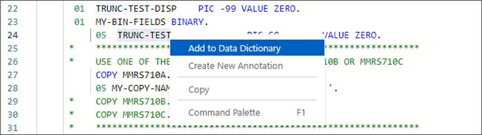
Step 2:
When the Data Dictionary Entry editor opens, in the Details tab, complete the fields below:
- Description: Enter a description for the data dictionary.
- Business-related: Select whether this entry is business-related.
- Optional text boxes: Completion of the Field Transformation, Source Input, and Target Output text boxes is optional.
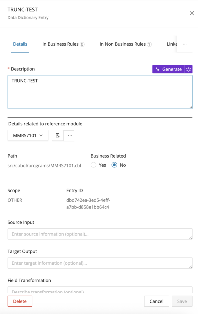
Step 3:
Click Save to save the data dictionary entry.
Editing Data Dictionary entries
Step 1:
To edit a data dictionary entry, hover the mouse over the entry in question and select Edit.
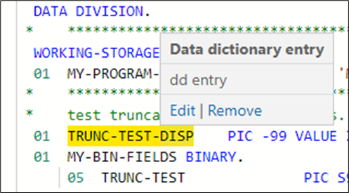
Step 2:
Make your edits in the window that opens. Any linked Annotations will be shown in the appropriate tab when opened in Code Viewer.
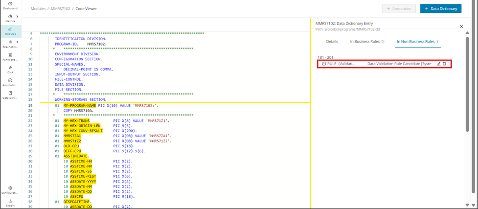
Step 3:
Click Save to save your changes.
Removing Data Dictionary entries
To remove a data dictionary entry, hover the mouse over the entry to be deleted and select Remove.
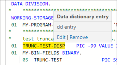
Data Lineage
You can also launch Data Lineage directly from the Code Viewer for supported fields and technologies. This is useful when you want to move from a specific source reference into a broader data-flow investigation. Follow the Data Lineage page for the CodeViewer for the complete workflow and visualization options.
Module Details
On the Modules page, click any Module Name in the table to display the corresponding mining data for that module on its Details page. This page centralizes the module's metrics, metadata, dependencies, and editing workflows in one place. Use it when you need a detailed view of a single artifact before moving into specialized tabs or visualizations.
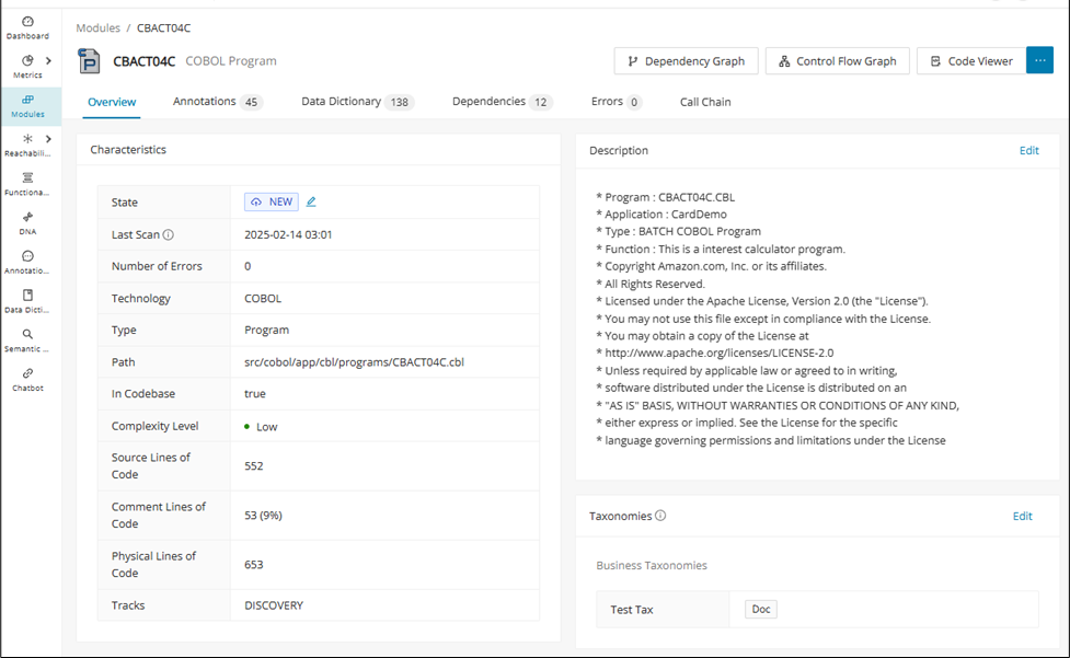
The following tabs are available to provide in-depth information about the selected Module:
| Contents | Description |
|---|---|
| Overview | The overview tab is divided into several panels: |
| Characteristics: Displays the characteristics of the module, such as state, language, type, path, whether the module is in the codebase, complexity, number of lines of code, and comment lines of code. | |
| Contained Module/Virtual Module: Indicates which virtual Modules are contained in the current one. If the current module is a virtual Module itself, the Virtual Module panel will display the Module that contains it instead. | |
Custom Properties: Allows for custom settings for Modules to fit the needs of each project. Click Edit Values to assign custom properties when none are assigned yet. For more information, see Custom Properties  |
|
| DNA (if available): Visualizes the data gathered by the Discover DNA feature for each module belonging to the same cluster. | |
| Control Flow Graph: Allows you to visualize the Control Flow Graph. For more information, see Control Flow. | |
| Dependency Graph: Visualizes the Dependency Graph, see Dependency Graph View. | |
Description: Enables you to add or edit the description of the Module. Click the Edit link in the description card to open the 'Edit Module Description' dialog.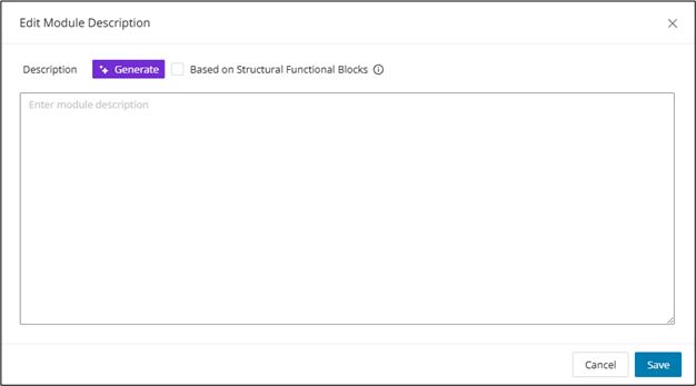 |
|
| Click Generate to populate the description text area with a Gen AI summary and check "Based on Structural Functional Blocks" if the description needs to be associated with the structural functional blocks. | |
| "Based on Structural Functional Blocks" only works for COBOL, and when used, existing structural functional block descriptions will be overwritten. | |
The feature toggle generativeAiTranslations must be enabled in the WebUI feature console. |
|
Taxonomies: The Taxonomies tab is only available if the project contains taxonomies. It displays all taxonomies assigned to this Module. Taxonomies can be directly assigned to the module by clicking Assign Taxonomies and selecting applicable values in the resulting overlay: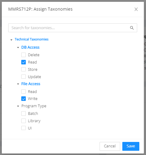 |
|
If taxonomies are already assigned, they can be edited or removed by clicking the Edit link: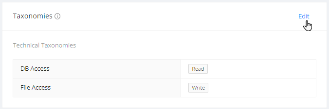 |
|
| Annotations | Lists and describes all assigned annotations for the selected module. The entries can be sorted and filtered by: Default Columns: - Annotation Type: Select a type from the drop-down menu - Category: Select a category from the drop-down menu - State: Select a state from the drop-down menu - Annotation Description: The description entered for this annotation - Source Code: The line(s) of code this annotation applies to - Modified By: The user who last updated the annotation - English Translation: The translation of the Source Code It is possible to customize the table by removing existing columns or adding other annotation-related columns to the table by clicking the settings icon on the right next to CSV . For example, it is possible to search, sort, or filter annotations by Business / Non-Business Variables Referenced, Process Sequence, Module Path, and Module Technology & Type. Each annotation entry can also be edited or deleted in an overlay window by clicking Edit on the far right of the table. A shortcut menu provides direct access to the Code Viewer for the corresponding module at the position of the selected annotation. Clicking CSV will download the table content in .csv format. |
| Data Dictionary | Lists all data dictionary entries for a module. It also includes data dictionary entries from the copy codes used. To filter by Field Name, start entering the first letters of the corresponding data element. - Module Name: Name of the module - Field Name: Displays the name of the field element - Field Type: Displays the field type - Field Description: Description of this field - Field Format: Displays the field format, for example, PICX or GROUP - Field Level: Level of this field - Group Field: Displays the group field - Length: Displays the number of characters in the data element name - Created By: The user who created the data element It is possible to customize the table by removing existing columns or adding other data dictionary-related columns to the table by clicking the settings icon on the right next to CSV . Clicking CSV will download the table content in .csv format. To learn more about conducting Field Level Mining from the Data Dictionary, access the Data Lineage page. |
| Dependencies | Lists all dependencies. You can filter by Target Name, Relationship Type, and Direction. To filter by target name, start entering the first letters of the corresponding dependency. - Target Name: Displays a list of target dependencies. - Relationship Type: The drop-down list can include the following types: CALLS, INCLUDES, READS_WRITES, REFERENCES. - Direction: The drop-down list offers the options IN and OUT. It is possible to customize the table by removing existing columns or adding other dependency-related columns to the table by clicking the settings icon on the right next to CSV . In the Dependencies tab, clicking Dependency Graph will open the Dependency Graph view. Clicking CSV will download the table content in .csv format. |
| Errors | Lists all related errors for the selected module. The table contains the following columns: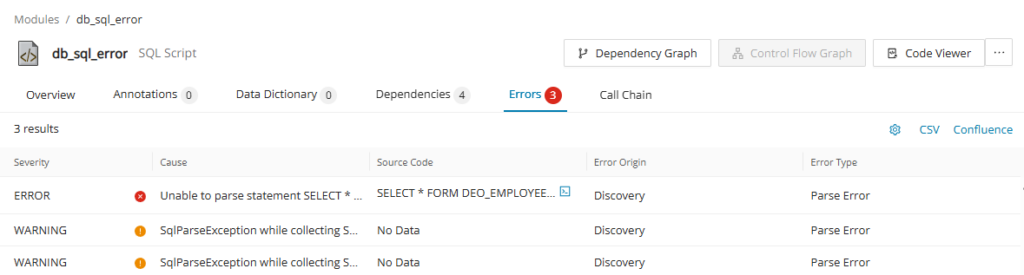 - Severity: Indicates the severity of the entry, whether it's an error or a warning. - Cause: Displays the error message and the cause of the error. - Source Code: If applicable, shows the source code where the error occurred. Click on to display a side panel "Marked Code" to see where the code has an error. 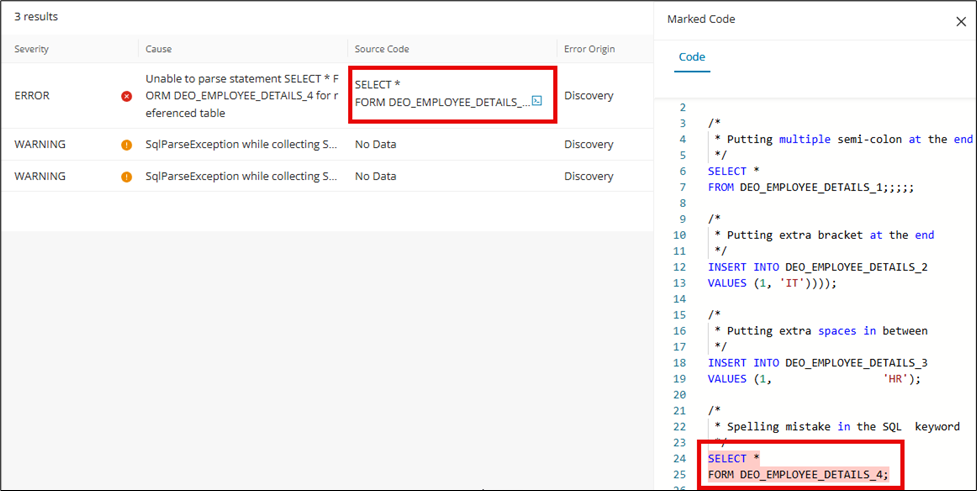 - Error Origin: Indicates the process in which the error occurred. - Error Type: Indicates the classification of the error: "parse error", "missing dependency", "internal error", etc. |
| Call Chain | Exports call chains in CSV with customizable properties for generating the call chain. See Call Chain for more information. |
Call Chain
The Call Chain feature allows you to analyze the in- and/or outbound sequence of modules and method calls referencing the currently selected module. The identified call chains are exported in .csv format with customizable properties for generating the call chain.
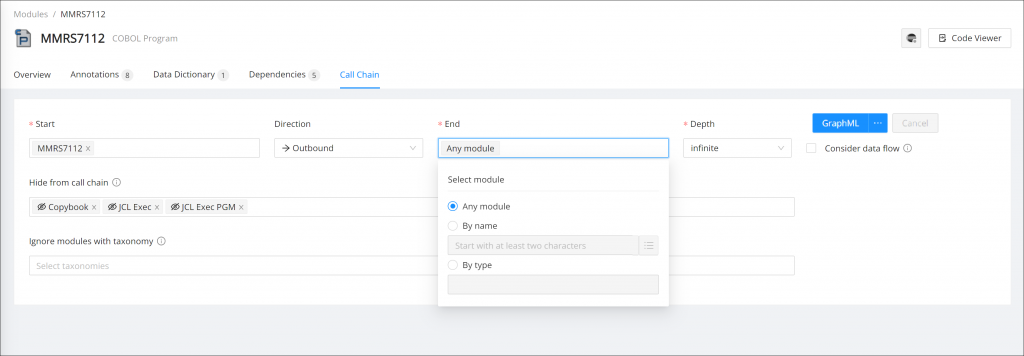
Call Chain has the following properties:
- Start: This field is filled out automatically with the Module on which you opened the Details page. This can be adjusted to any other module as the starting point of the call chain.
- Direction: This field determines whether inbound, outbound, or both modules are included in the call chain analysis.
- End: Mandatory. This field is filled out automatically with the default value "All Modules". This can be adjusted to any other module as the termination point of the call chain.
- Click the Start or End field to see the available options.
- All entry point modules/All Modules: The default entry for the End field. If the Start and/or the End field value is cleared, it is automatically populated with this option.
- By Name: Select this option to search for the modules by name. Select the input field to display a list of the available modules. You can select any number of names in the list.
- By Type: Select this option to search for the modules by type. Click in the By Type field to display a list of all available types. You can select any number of types in the list. Selecting a combination of modules from the options By Name and By Type is also possible, for example, to generate the call chain between a specific module and all BMS Map programs.
- Depth: Select the depth of the call chain. By default, Depth is set to "infinite".
- Format: Select your desired export format (GraphML, CSV, ZIP, or CSV)
- Hide from call chain: Optional. By default, the types "COBOL Copybook", "JCL Exec", and "JCL Exec PGM" are hidden from the call chain export. Click in the Hide from Call Chain field to display a list of all available types. You can select any number of types to exclude from the call chain results.
- Ignore modules with taxonomy: Optional. This field allows you to select any of the available taxonomies in your project. If a module with a selected taxonomy is detected in the call chain analysis, the module itself will be included in the call chain, but its subsequent in- and outbound dependencies will be omitted.
Edit inserted modules
After selecting the modules in the start/end field, click Edit Selection to open the "Insert Module List" dialog. To remove the already inserted modules from the "Insert Module List" dialog, click the at the end of the selected row of modules.
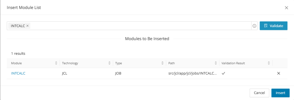
After removing the desired module/s from the list click Insert and the start/end field will be updated to the reduced module count.
Call Chain visualization
Hone the Call Chain options to your liking and click Render Graph to produce the Call Chain Visualization.
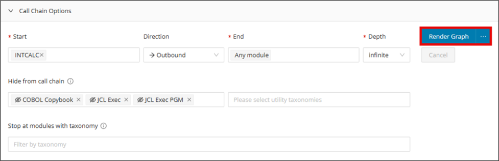
The visualization of the call chain can prove to be useful in understanding the in- and/or outbound sequence of modules and method calls.
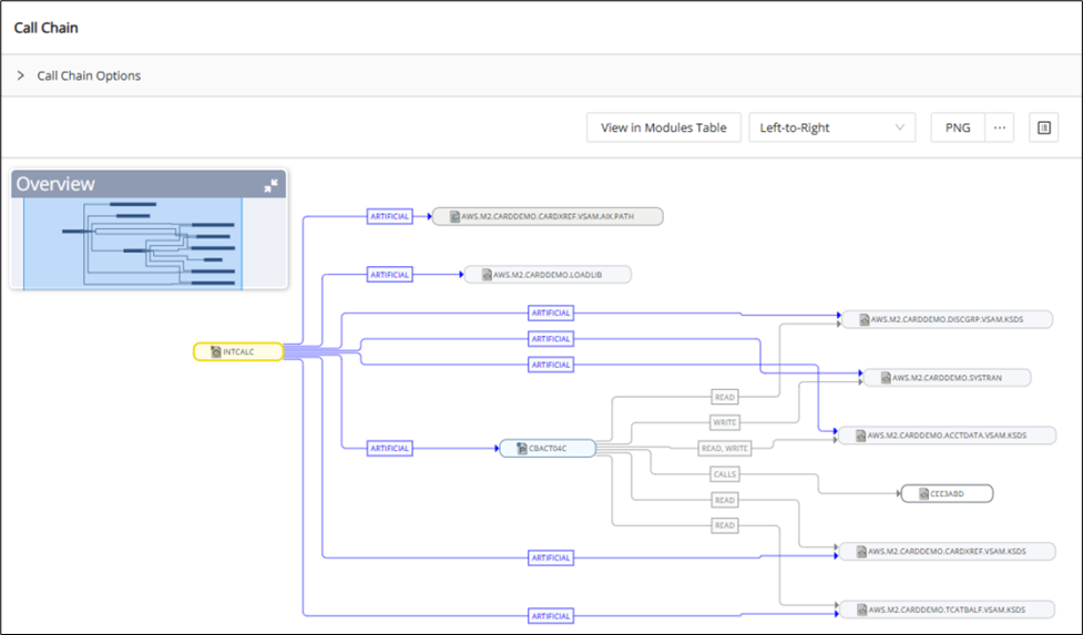
Manipulate the call chain visualization with the following features:
- View in Modules Table: Open a tab to the included Modules Table
- Visualization Layout: Select from a drop-down menu to change the layout of the visualization 1. Hierarchical 2. Left-to-right 3. Organic 4. Balloon 5. Radial 6. Cyclic
- Export: Export the call chain visualization as a PNG, GraphML, PDF, or SVG
- Toggle Side Panel: Toggle on or off to open an informative side panel to find more details on any node or edge. The side panel for nodes gives the option to Open Control Flow, Open Dependency Graph, Open Code Viewer, or Open Module Details for the selection.
Artificial edges
Artificial Edges are used to condense the graph when certain modules with specific Technologies, Types, Utility Taxonomy assigned, or Dependency Relationships are filtered/hidden. Edges represent the dependency connection between two module nodes on the graph. These edges in dark blue signal that there are modules and/or additional edges between one module node and another; however, they were manually hidden versus other modules displayed along the graph.
Creating artificial edges
Expand the Call Chain Options dropdown, and in the "Hide from call chain" field, there are several default types set to be hidden by default, including COBOL Copybook, JCL Exec, and JCL Exec PGM. These will automatically create artificial edges on the graph when these types of modules are encountered; however, you can add additional technologies, types, or modules assigned utility taxonomies you would like to be hidden and shown only as part of an artificial edge. To remove artificial edges, simply remove associated unwanted selections from the "Hide from call chain" field.

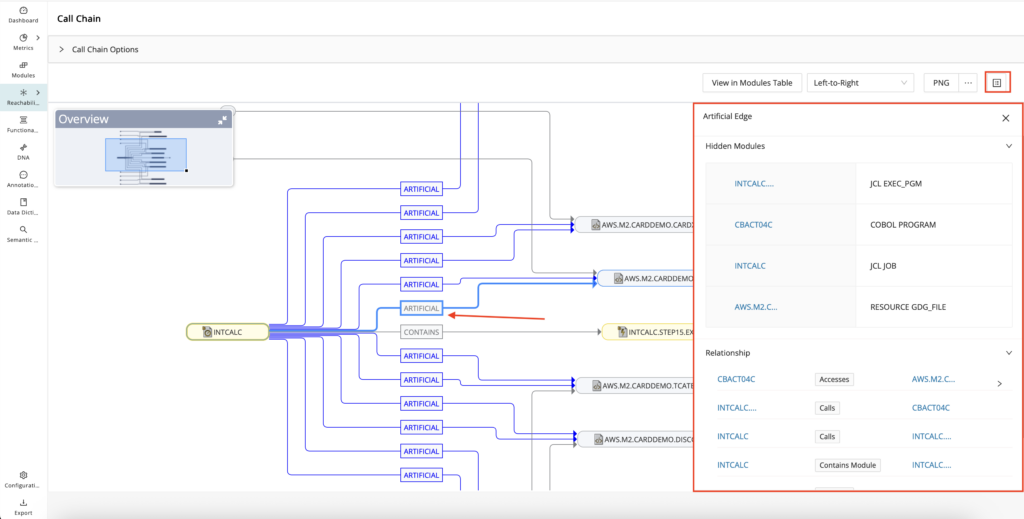
Info
Artificial edges are rendered from both the Call Chain and Dependency Graph, where you can filter technologies, types, edges, and modules with utility taxonomy assignments.
Shared Module Details side panel

From the Call Chain Graph, click on your module node of interest and click on the side panel icon.
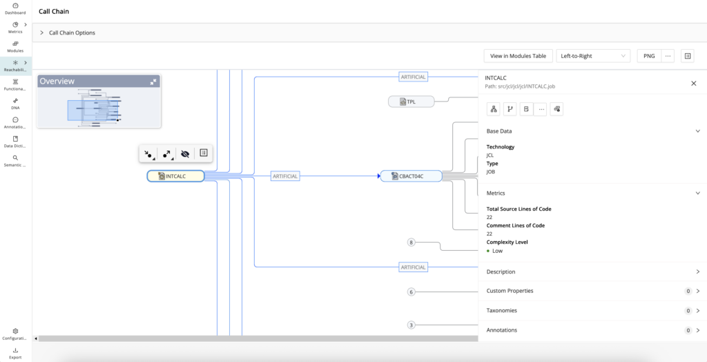
Edge side panel
From the Call Chain Graph, click on the edge representing the dependency relationship between two modules (includes artificial edges) and click the side panel icon on the top right next to the PNG export button.
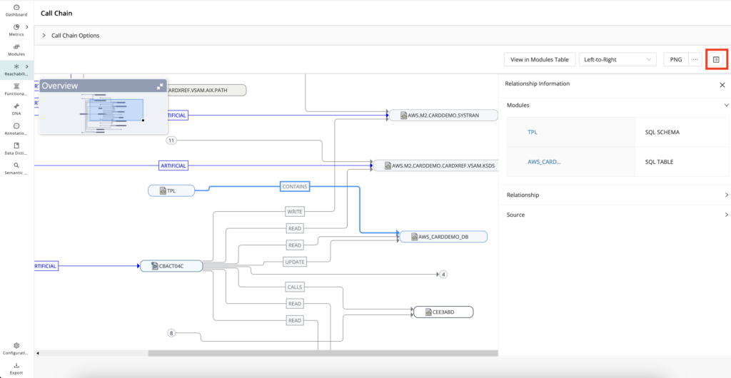
Dependency Graph
The Dependency Graph view uses yFiles for visualizing application dependencies. yFiles is a library for the visualization and automatic layout of graph structures.
To display the graph from the Module Details, click Dependency Graph .
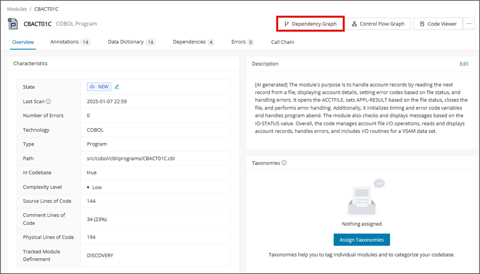
The Dependency Graph view allows you to filter the dependencies displayed, set the display depth, and select the layout style used. At the top of the view, three drop-down lists provide filtering options for the graph. The titles of the drop-down lists are updated to reflect your filtering selections. To save the Dependency Graph, select the desired format from the menu on the top right of the view. You can choose from PNG, PDF, SVG, or GraphML.
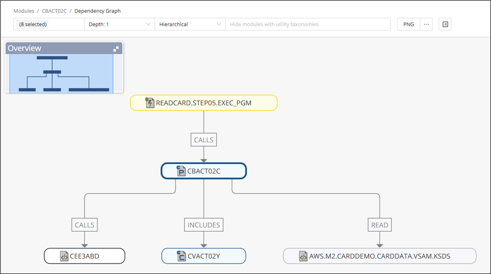
Drop-down list for selected
This filter allows you to select the items to display. The title of the drop-down list displays the number of items selected, for example, "7 selected". If you filter nodes that have a transitive dependency, the edges will be merged into one new edge so that the dependency to the transitive referenced node is still displayed.
Info
A transitive dependency is an indirect functional dependency, that is, any dependency that is induced by the components that the program references directly. For example, a call to a log() function will usually induce a transitive dependency on a library that manages the I/O to write the log message in a file.
From the drop-down list, deselect the nodes that you wish to omit. (In our example, it is JCL EXEC PGM.) Subsequently, the deselected nodes are displayed in white.
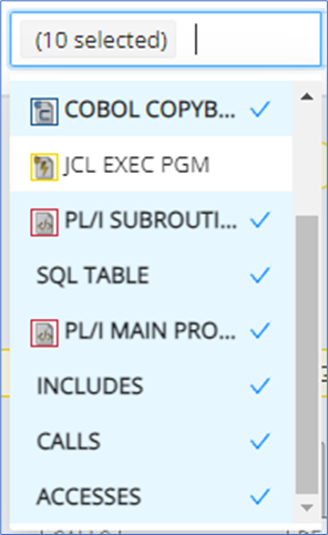
Depth: < > drop-down list
Allows you to select the depth (level) of the dependencies displayed. Depth range: 1 - 10.
Hierarchical drop-down list
Allows you to visualize the hierarchy with the following layout styles: Hierarchical (default), Left-to-Right, Organic, Balloon, Radial, and Cyclic. The layout style selected is displayed as the title of the drop-down list.
Filtering the edges of nodes
An edge filtering feature allows users to selectively enhance the depth for specific nodes without having to change the depth for the entire dependency graph. Simply click a node to display a context menu, which allows you to select/deselect the edges you wish to display. For example, you can display only the outgoing or incoming calls for a node.
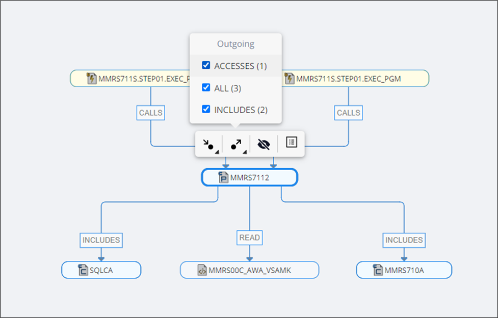
This feature makes working with the dependency graph more productive, and users can focus on areas of interest on the graph.
| Icon | Description |
|---|---|
| Clicking a node and selecting the Incoming Edges icon from the context menu will display a list of nodes that can be deselected. If the selected node has no incoming edges, the message "There are no incoming edges for this node" will be displayed. | |
| Clicking a node and selecting the Outgoing Edges icon from the context menu will display a list of nodes that can be deselected. If the selected node has no outgoing edges, the message "There are no outgoing edges for this node" will be displayed. | |
| To hide a node, click the Hide Node icon. Root nodes cannot be hidden. If you click a root node and select the Hide Node icon from the context menu, the message "Root node cannot be hidden" will be displayed. | |
| Select Open Side Panel to open the side panel for the selected module. |
Toggle side panel
When Toggle Side Panel is selected, the side panel will open and stay open. When the user switches between edge and module information, the side panel will be dynamic and change information based on what is selected.

Another way of opening the side panel is by clicking the module and selecting Open Side Panel from the context menu displayed.
The side panel of the selected modules displays the module name, path, base data consisting of technology and type, metrics, description, custom properties, taxonomies, and annotation.
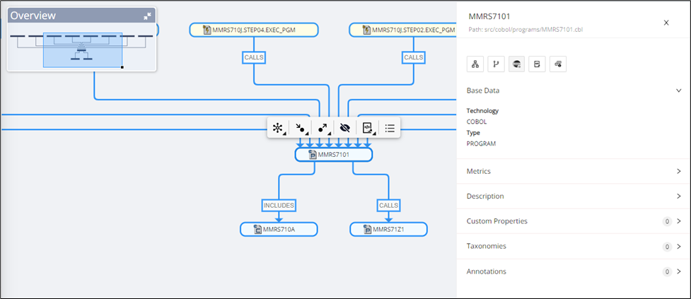
| Icon | Description |
|---|---|
| Open Control Flow | |
| Open Dependency Graph | |
| Open Code Viewer to open and review the selected module's source code | |
| Extends Open Code Viewer with options to view Single or Assembled Module View | |
| Open Module Details |
The edge side panel displays the relationship information, such as modules, relationships, and source code, when the edge is clicked.
| Edge Side Panel Information | Description |
|---|---|
| Modules | Shows the two modules of the edge and their associated technology and type of file |
| Relationship | Shows the specific interaction or dependency type between two modules |
| Source | Shows the source code of the edge |
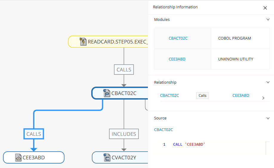
The relationship information will also display all of the relationships between two modules, for example, if a module calls another module multiple times.
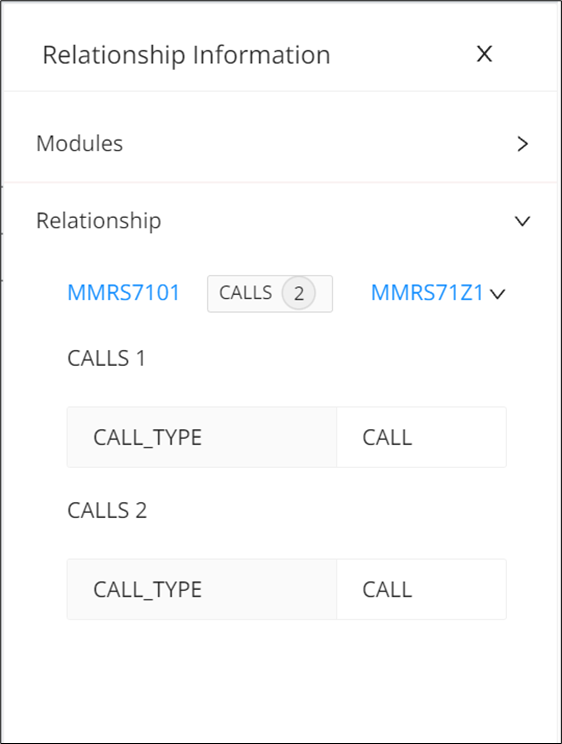
File record layout
The edge side panel also includes a feature called "File Record Layout," which details how the data in the file is structured (extracted from the COBOL module) for access type details. Also, there can be multiple file record layouts on the same file based on the different modules accessing it.
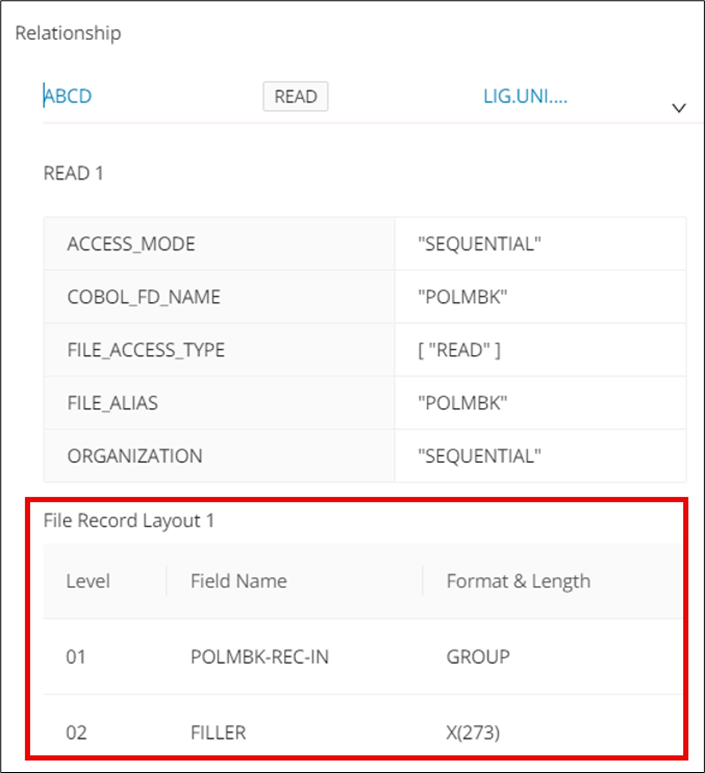
Shared Module Details UI component
Info
This feature is available not only from the Dependency Graph but other graphs as well including the Call Chain, Data Lineage, and Reachability Details Graphs.
The shared module details component provides quick access to module details wherever you are in the UI, without the need to navigate back to the Module Details page. Clicking a module reference, that is, a node in the dependency graph, will open a dialog showing all relevant module details.
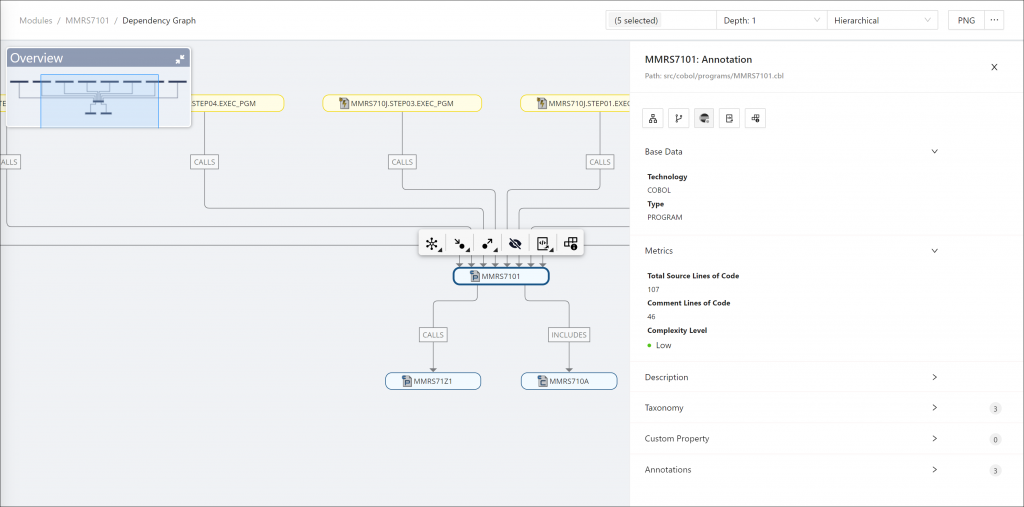
Control Flow Graph
You can visualize the executable control flow of a program in a graph, and for COBOL, you can extend this to see the control flow beyond your program to visualize called programs within the context of the same graph. To calculate and view the control flow graph, click Open in the Control Flow Graph card.
Info
This feature fully supports C, COBOL, JCL, Natural, and PL/I, and has partial support for Java.
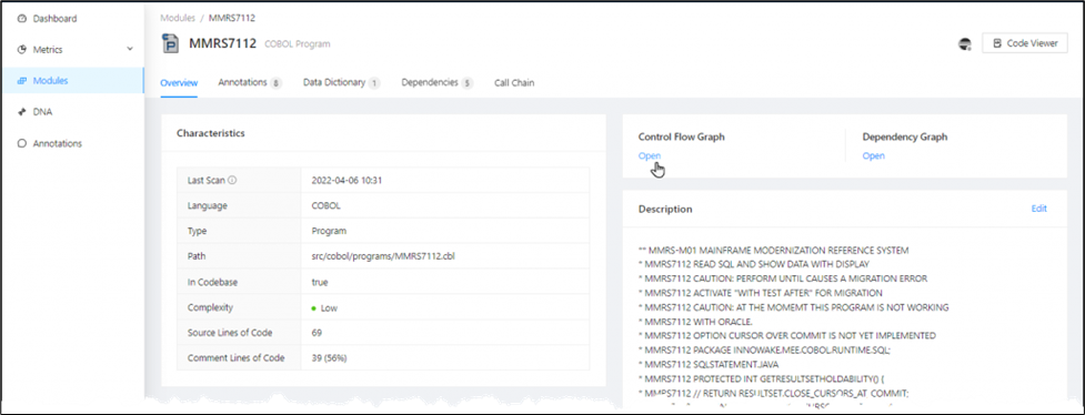
The nodes in the graph have the following meaning:
- Circles represent the entry and exit points of the program.
- Rectangles represent executable action statements.
- Rhombuses represent conditional statements.
A 20-character limit is applied to the texts in each node. If the text exceeds that limit, it will be truncated with three dots (...). Edges of conditions are labeled with true or false.
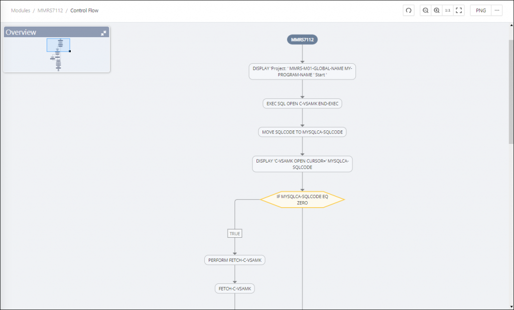
Toolbar actions
The toolbar contains icons for resizing the contents and options for saving the graph:
| Icon | Description |
|---|---|
| Click the Recalculate icon to reset the graph to its original state. | |
| To zoom out of the control flow graph, click the magnifying glass with the minus sign. | |
| To zoom in on the control flow graph, click the magnifying glass with the plus sign. | |
| Click 1:1 to zoom to the original size. | |
| Click the Fit Content icon to resize the control flow graph to fit the window. | |
| To save the control flow graph, select the desired format from the drop-down menu. You can choose from PNG, PDF, SVG or GraphML. |
The Control Flow Graph page displays an error message if the calculation of the control flow graph failed and no content was generated. The error message contains a link that opens the Error tab on the Module Details page.
Core operations icons for Cobol programs
The control flow for Cobol programs provides the following icons next to the nodes that signal core underlying operations to quickly identify nodes of significance on the graph.
| Icon | Core Operation |
|---|---|
| File Read / Write / Open / Close | |
| Database Open / Read / Fetch / Close | |
| Compute Operations | |
| Program Calls | |
| Annotations |
Collapsible Control Flow graph
Info
This feature is currently available for COBOL only.
Sections, paragraphs, and branches of the control flow graph are grouped in expandable panels that are collapsed by default. Each panel can contain additional expandable panels, depending on the complexity of the grouped element.
Select the and icons in the block's top right corner to expand or collapse the panel, respectively. To expand all panels at once, click Expand groups in the top menu bar. To collapse all panels at once, click Collapse groups in the top menu bar.
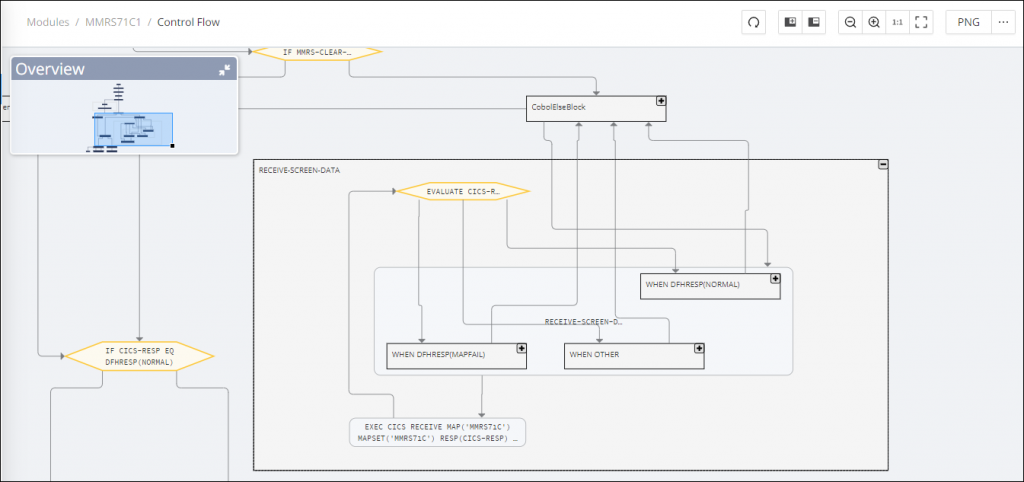
There is no collapsible control graph for a group node that contains only a single node. In this case, only the child node will appear instead of the parent node.
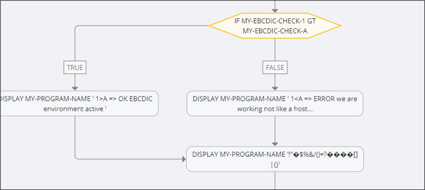
Expanding the Control Flow graph
Info
This feature is currently available for COBOL only.
Call statement nodes that transfer executable control to an external module can also be loaded and then expanded/clicked to generate and visualize the control flow for the external module as well.
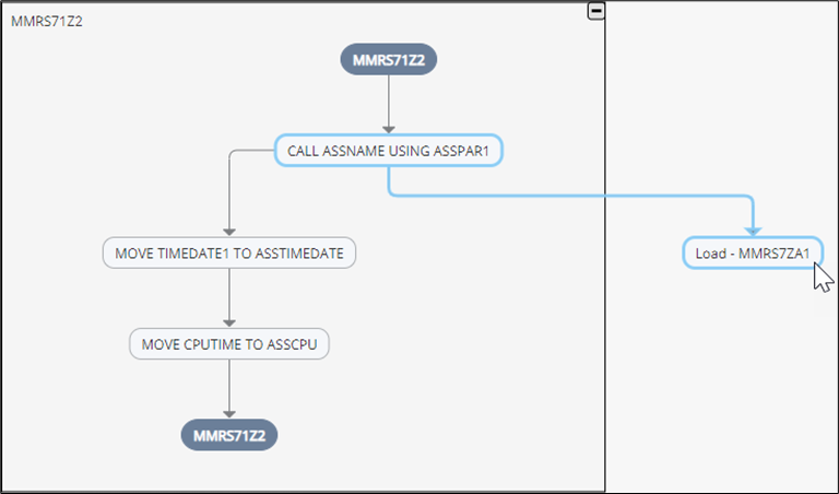
Highlighting the Control Flow graph
Hovering the cursor over or clicking any node in the control flow graph highlights other nodes that are connected to the clicked node. Hovering over a node will highlight the nodes in light blue, and clicking a node will highlight the nodes in dark blue. Clicking outside the graph will remove the previous highlighting of the nodes.
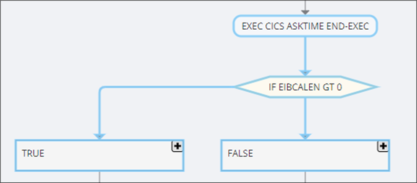
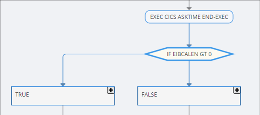
Source code panel
Some modules have a large control flow graph, and the order of the nodes can be confusing at times. For this reason, when you click any node in the control flow graph, the source code is displayed in the pane to the right of the graph, with the specific source code of the clicked node highlighted with the line position.
Clicking the node with the module name (for example, "MMRS7101") displays the whole source code. The name of the clicked node is also displayed as a header in the source code.
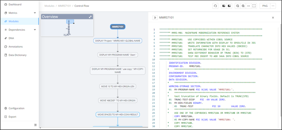
Clicking a specific node displays the source code in such a way that the code associated with the node is highlighted together with the corresponding header and line position.
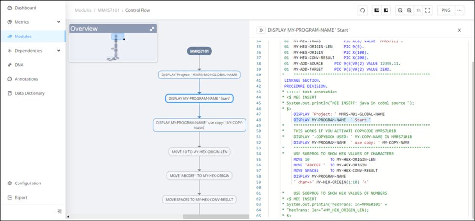
Clicking a collapsed group node displays the source code in such a way that all lines of code within the selected group node are highlighted.
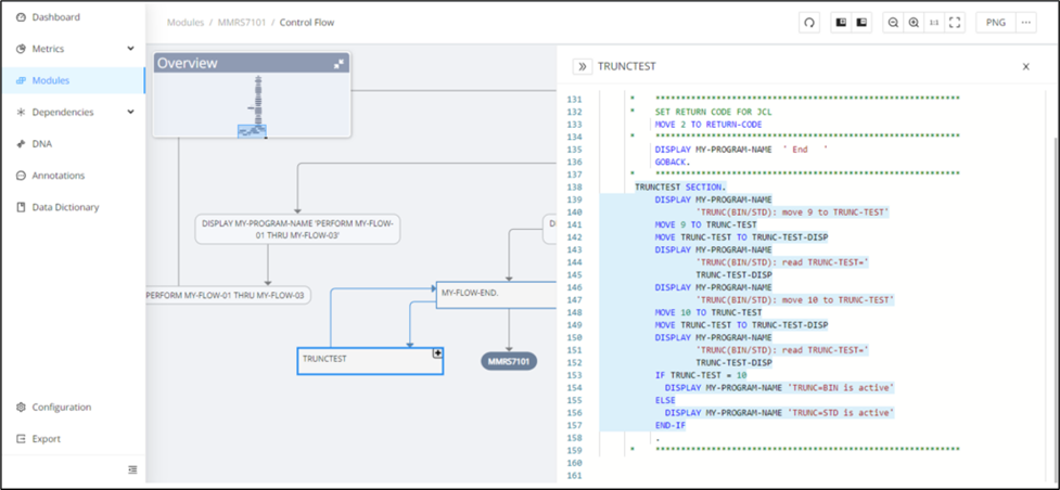
Highlight Annotations
This feature highlights the annotations to distinguish the unique execution path for modules with identified business rules on the Control Flow Graph page.
The Control Flow Graph for the module with identified business rules will be displayed as "Business Rule Candidate [System identified]" as a separate AST node in a blue dashed border with a expand icon at the top right corner of the node.
Click to expand the node and display a side panel highlighting the annotation's source code.
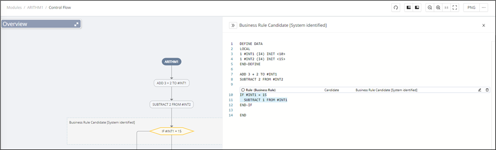
In addition, the Annotation editor contains a Control Flow graph that redirects to the Control Flow Graph page zoomed to the selected annotation.
The source code tab should contain both the annotation block and the annotation node. To access the annotation block, click the node for the source code tab. The annotation block can be edited and deleted as needed, and the same will be reflected in the control flow graph. Click Edit to display the annotation editor and edit the type, category, annotation description, and state of the annotation.
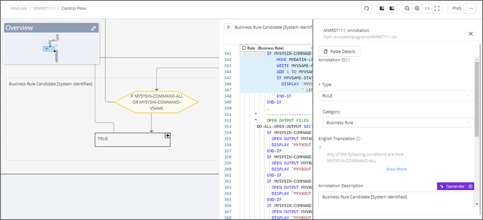
If needed, click Delete to completely remove the annotation from the source code.
Control Flow process grouping
For sequential statements that do not branch or jump to other parts of the program, they are grouped into what's called a process to further abstract the graph and reduce the visual clutter so that you can see as much of the bigger picture of the overall flow of the program by default, and dig into the details as needed.
Info
This feature is currently available for COBOL only.
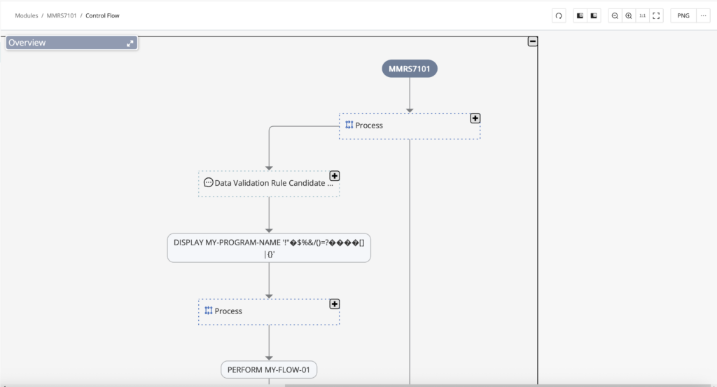
Code Viewer
The module code can be reviewed by clicking Code Viewer in the top right corner (opens Assembled View by default). Hovering over the three dots gives the option to view in Single Module View or Assembled View. The Code Viewer also offers Annotation and Data Dictionary editing in the Web UI. For those workflows, see Code Viewer.
Custom module table state
After switching between tabs on the Module Details page, the customizable state of the filters, sorting, and columns remains the same. This persistent state makes it easier to compare related information across tabs without rebuilding the same table view. Use it when you want filters and visible columns to carry over as you move between module details tabs.
Example:
Choose a Module and click it, and that will navigate to the Annotation Tab. Created Annotations are displayed, after that, customize the state of the Tab:
- Filter Annotations Type with DATABASE and State with CANDIDATE;
- Click the settings icon and add a Path column.
- After that, click the Data Dictionary Tab.
The filters and columns remain the same.

Info
After refreshing the page, the state changes to default.
Reachability Analysis
To help understand and structure the technical dependencies of a system, Code Discovery & Mining offers analysis via Reachability blocks. Reachability blocks represent a dependency graph from one upper bound (like a job or stored procedure) to its lower bounds (like a table or file) via the modules in between the bounds. Reachability blocks can be easily created automatically based on desired criteria and analyzed from the overview of the Reachability page.

Reachability analysis form groups of modules by following the call chains between defined upper bound and lower bound modules.
Access control on Reachability Block view:
-
Viewer: Cannot modify anything on a reachability screen, that is, can only view the reachability blocks. Does not have permission to edit or rename the reachability blocks.
-
Editor: Can modify and edit the reachability block and screens, but cannot perform any bulk operations, that is, bulk delete reachability blocks or perform reachability analysis.
-
Manager: Has full access, including bulk operations like re-running reachability analysis or bulk deleting blocks.
| Operation | Viewer | Editor | Manager |
|---|---|---|---|
| Create Reachability blocks and perform analysis | No | No | Yes |
| CSV export of the Reachability Block details table | Yes | Yes | Yes |
| Filter Reachability Block based on Taxonomy | Yes | Yes | Yes |
| View details of a Reachability Block | Yes | Yes | Yes |
| Customize the column of the Reachability Block details table | Yes | Yes | Yes |
| Switch the upper/lower bound of the Reachability Block details table | Yes | Yes | Yes |
| See all nodes in the modules table of the Reachability Block details table | Yes | Yes | Yes |
| Edit the name and description of a reachability block | Yes | Yes | Yes |
| Show/Hide inactive reachability blocks from the overview screen | No | Yes | Yes |
| Merge/Unmerge Single Reachability Block | Yes | Yes | Yes |
| Activate/Inactivate Reachability Block from inside the RB details screen | No | Yes | Yes |
| Merge/Unmerge Single Reachability Block | No | Yes | Yes |
| Bulk Inactivate Reachability Blocks | No | No | Yes |
| Single Recalculation | No | Yes | Yes |
| Bulk Recalculation | No | No | Yes |
| Access Successor/Predecessor graphs | Yes | Yes | Yes |
| Configure Technology & Type for RB | No | No | Yes |
Create Reachability Blocks
To begin reachability analysis, navigate to the Reachability page to create reachability blocks. If there are no reachability blocks created yet, the Reachability page introduces reachability blocks as below. The creation flow lets you define the boundary criteria that determine which end-to-end paths are grouped together.
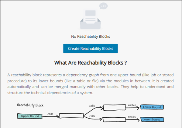
When you are ready, click Create Reachability Blocks to begin reachability analysis. The following pop-up window gives the option to perform reachability from the following criteria:
-
Upper or Lower Boundary (select from the radio buttons on the top left)
-
Technology & Type (configure this by clicking the settings icon, more info under Technology & Type Configuration)
-
Taxonomy
-AND/OR logic for multiple taxonomies
-Tooltip: If no taxonomy is selected, then all upper/lower bound types will be selected for analysis
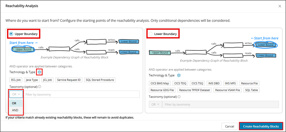
After filling in the desired criteria, click Create Reachability Blocks to complete the reachability analysis. After the reachability analysis is complete, the Block View will automatically populate itself with reachability blocks. To create more reachability blocks, click + Add Reachability Blocks in the top right corner.
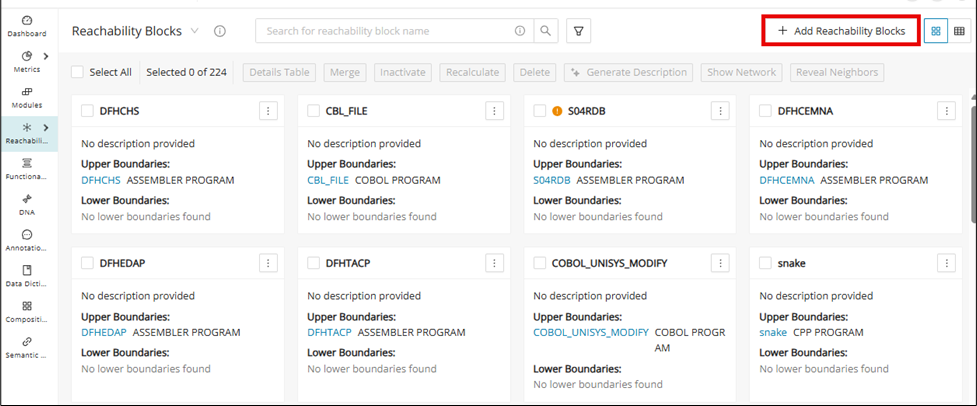
Technology & type configuration
Info
Only users with the following roles can edit the Reachability configuration: Admin, Client-Admin, and Managers. Viewers and Editors are restricted from performing these configurations.
When creating Reachability Blocks, you can edit the default Technology and Types that come with their creation. To do this, either:
- Navigate to the Configuration page and click the Reachability tab or
- Navigate to the Reachability page and click Add Reachability Blocks and then click Edit
You will then see the default Technology & Type that are associated with the Upper and Lower Boundaries.
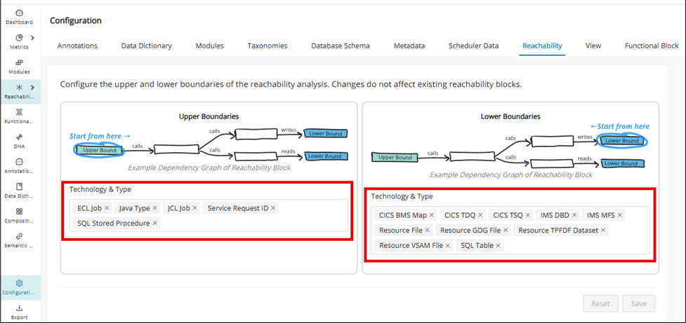
Either add or remove Technology & Type and then click Save to save the settings for future-created Reachability Blocks. All changes that are made can be reverted by clicking Reset while making changes.
UI validations
Warning
The Technology & Type of the Upper and Lower Boundaries must contain at least one item; otherwise, an error message will be displayed.
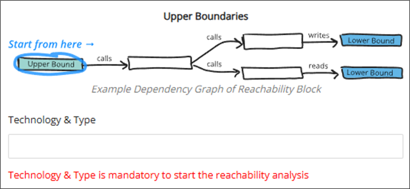
Warning
The Technology and Type in Upper and Lower Bound cannot be the same; otherwise, end-to-end flows cannot be determined, and the following error message will be displayed.

Reachability Analysis results
With reachability blocks now created and visible on the Reachability Blocks page, you are ready to conduct Reachability Analysis. This section provides an overview of the available features designed to help you understand the technical dependencies of your system. From here, you’ll learn how to leverage these tools to gain deeper insights into application structure and behavior.
Block view
After the reachability analysis, the Block View displays all reachability blocks in a grid. A reachability block represents a dependency graph from one upper bound (like a job or stored procedure) to its lower bounds (like a table or file) via the modules in between. This is created automatically and can be merged manually with other blocks. They help to understand and structure the technical dependencies of a system.
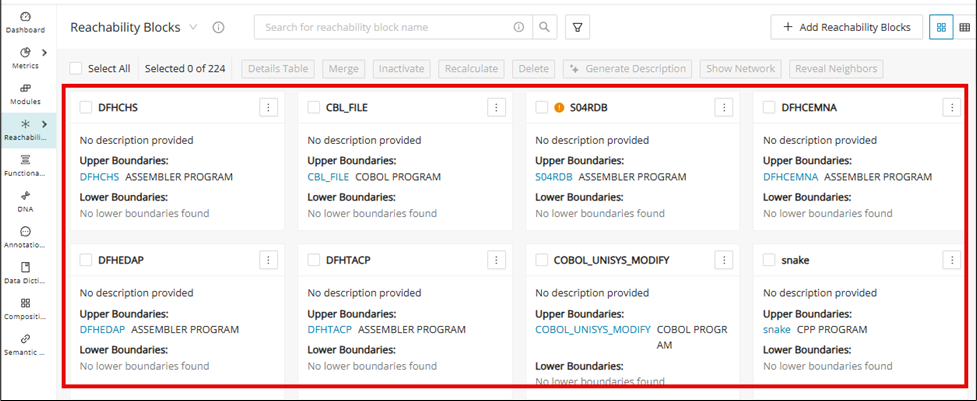
Toolbar
| Button | Description |
|---|---|
| Details Table | Opens Details Table for selected reachability block(s) |
| Merge | Merges selecting reachability blocks |
| Inactivate | Inactivates selected reachability block(s) |
| Recalculate | Opens a visual network view of the selected block(s), connections, and dependencies |
| Delete | Removes the selected reachability block(s) from the project. |
| Generate Description | Automatically creates a summary or explanation for the selected block(s) |
| Show Network | Opens a visual network view of the selected block(s), connections, and dependencies |
| Reveal Neighbors | Displays modules directly connected to the selected reachability block(s) |
Table view

The default view for the reachability blocks page is Block View. To instead view all of the reachability blocks in tabular form, toggle from the Block View to the Table View in the page header.
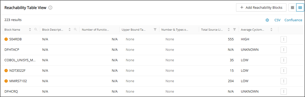
Reachability Block details
Within the Block View, the summarized details are shown in each reachability block. To find more detailed information within a reachability block, click any reachability block.
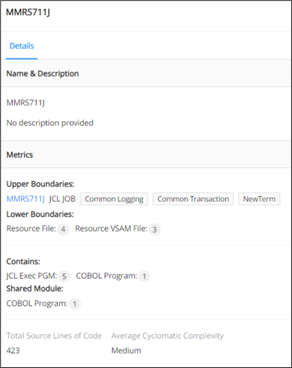
-
Name & description
-
Metrics
-Displays the upper and lower boundaries and their technology, types, count, and other details.
-Shows the relationships with other modules and what is contained within the reachability block. -
Total source lines of code:
-Represents the total lines of code for all modules within a reachability block, including upper and lower bounds and everything in between.
-For merged reachability blocks, the total lines of code updates automatically when blocks are added or removed.
-The total lines of code for a merged reachability block are the sum of all its blocks. -
Average cyclomatic complexity:
-Displays the average cyclomatic complexity for all modules within a reachability block, including upper and lower bounds and everything in between.
-For merged reachability blocks, the average cyclomatic complexity updates automatically when blocks are merged, unmerged, added, or removed.
-The average cyclomatic complexity for a merged reachability block is the average of the complexities of all its blocks.
Removed Reachability Blocks
When upper bounds can't be found or deleted, then the whole reachability block with those upper bounds will cease to exist. This feature allows you to have a chance to review removed blocks with the possibility of restoring them by providing a notification before total removal.
Single Reachability Block containing deleted upper bound module:
-
Visual indication:
-Deleted reachability blocks will be marked with a delete icon -
Menu and tooltip:
-Menu items for deleted blocks will be disabled.
-Hovering over these items will show a tooltip: “The Upper boundary was removed. Not possible to edit or view details.” -
Notification and dismissal:
-A message at the top of the screen will state: "Some reachability blocks were removed because of missing upper boundaries. You can dismiss them."
-Click Dismiss Removed to remove these blocks from view. -
Pagination:
-The notification banner will appear on all pages until dismissed.
-Dismissing the message removes all deleted blocks from all pages. -
Checkbox visibility:
-Rows with removed upper-bound modules will not have checkboxes.
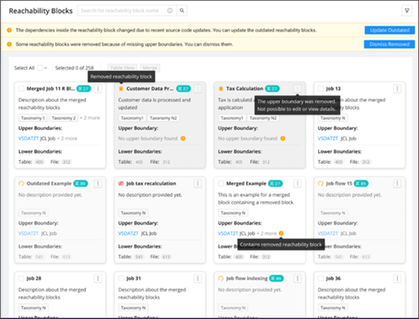
Merged RB containing a deleted Reachability Block:
-
Indicator for deleted Modules:
-If any upper-bound module in a merged reachability block is deleted, an indicator will be shown on the overview screen instead of marking the entire block as removed. -
Details view:
-In the blocks tab of the Details view, deleted reachability blocks will be displayed.
-Click Dismiss Removed to remove these deleted blocks from the screen.
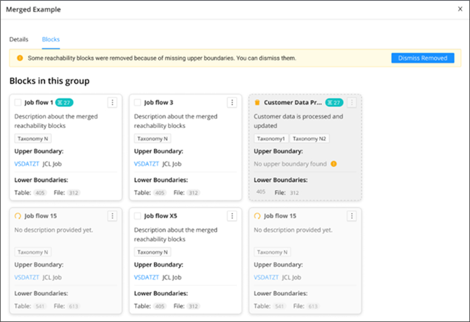
-
Checkbox availability:
-If a merged reachability block has at least one active upper bound module, the checkbox will be enabled, allowing it to be available for merging. -
Merging with removed Modules:
-When merging a merged reachability block containing removed upper bound modules with another block, the same indicators and messages will appear in the newly formed merged block.
-
Display of fully removed blocks:
-If all upper-bound modules in a merged reachability block are removed, the entire block will be shown as removed. -
Details table:
-The Details Table will only display details of available upper-bound modules, not the deleted ones.
-A banner will indicate: "Some reachability block details were not populated in this table because of missing upper boundary(s) due to source code updates or may have been deleted manually." -
Dismiss removed functionality:
-If a merged block contains two blocks and one is removed, clicking Dismiss Removed in the Details view will remove the deleted block.
-If only one block remains, the merged block will revert to an unmerged state, adopting the name of the remaining block.
Deleted Reachability Blocks Details Graph:
-
Deleted Reachability Blocks:
-No Details Graph will be available for deleted reachability blocks.
-Menu items for deleted blocks will be greyed out and disabled. -
Merged Reachability Blocks:
-For merged blocks containing deleted reachability blocks, the Details Graph will exclude modules from the deleted blocks.
-The graph will display links and paths only between the modules of the existing blocks within the merged block.
Auto detect outdated Reachability Blocks
This feature indicates when an existing reachability block is outdated. If the source code is modified, then the whole reachability block will be marked as outdated. In that case, we will provide a notification to the user indicating that the block has been outdated and needs recalculation.
Single and merged outdated blocks
The outdated blocks in the cards in the overview screen will be indicated with an outdated icon in place of a checkbox, and a tool tip message, as shown below
You will be notified when a re-calculation/re-run of the reachability analysis is needed, with an alert on top of the screen whenever there is at least 1 outdated reachability block.

This banner will be visible on all of the pages in case of paginated data, until updated. Click Update Outdated to retrigger the reachability analysis. The page loader will be displayed in case it takes time to run the reachability analysis after clicking Update Outdated.
In the case of a Merged RB, if any one of the included blocks is outdated, the merged block will be shown as outdated. If a block is inactive, there will be no check for whether the block is outdated.
This will also work with pagination. For example, if there is 1 outdated block in the 2nd or 3rd page and you are on the 1st page, the outdated banner, along with the Update Outdated button will still be displayed on every page.
The banner will appear in the following:
-
The Reachability Block card view
-
The Reachability Block details if the block is merged and contains outdated blocks
-
The Reachability Block Table details whether the block is merged and contains outdated blocks. Show in all pages, in case of paginated data
-
The Reachability Block Table details if the block is single, but it contains outdated modules
-
The Reachability Block Details Graph, that the block is single and contains outdated modules.
-
The Reachability Block Details Graph, that the block is merged and contains outdated blocks.
The Update Outdated button will only be visible to users with the key cloak roles: Editor, Manager, and Admin.
Viewers can only view the banner and cannot see the Update Outdated button.
Edit name & description
Generate a single Reachability Block description using Gen AI
Configuration
To use this feature
1. Enable the generativeAiTranslations feature toggle.
2. Module description should be available for the modules available in the reachability blocks.
Step 1:
Navigate to the Reachability Blocks overview screen, click the menu icon of a Reachability Block, and then click Edit Name and Description .
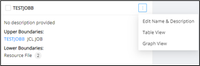
Step 2:
Click Generate to generate the reachability block description.
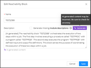
Step 3:
Click Save to save the description, and it can be seen on the RB overview and the view details screen.
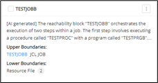
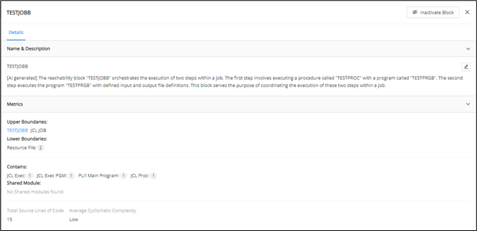
Reachability block descriptions can be generated from the View Details screen as well.
Step 1:
Click any reachability block on the reachability blocks overview screen.
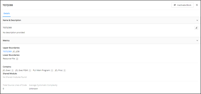
Step 2:
Click the edit icon to edit the name and description
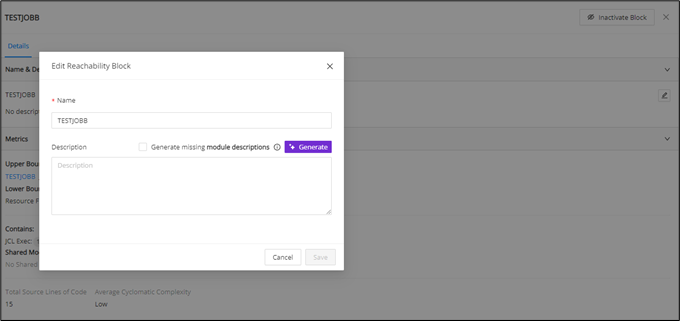
Step 3:
Click Generate to generate the description.
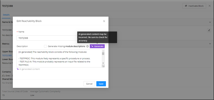
Details graph
Details Graph for an individual Reachability Block
Navigate to the Reachability Blocks window and click the menu icon of the respective reachability block.
Click Details Graph from the menu.
The Details Graph of the modules present in the selected reachability block is displayed as shown in the following figure. The upper bound module is displayed on the left and points to the lower bound modules on the right.
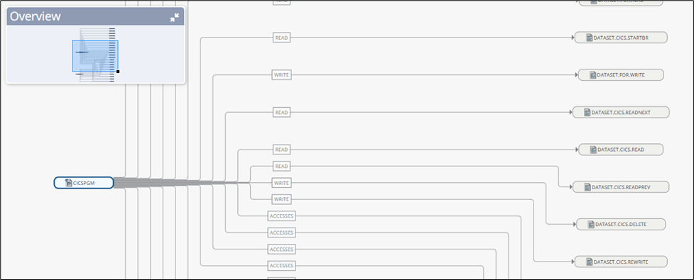
Details Graph for a merged Reachability Block
For a merged reachability block, click the menu icon. Then click Details Graph from the menu.
The Details Graph for a merged reachability block is displayed as in the following figure.
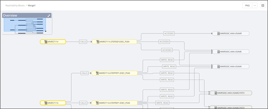
Filter for Details Graph for individual Reachability Blocks
Filter individual reachability block graph modules using "Taxonomy", "Technology & Type", "FB", and "Reference Types" between modules.
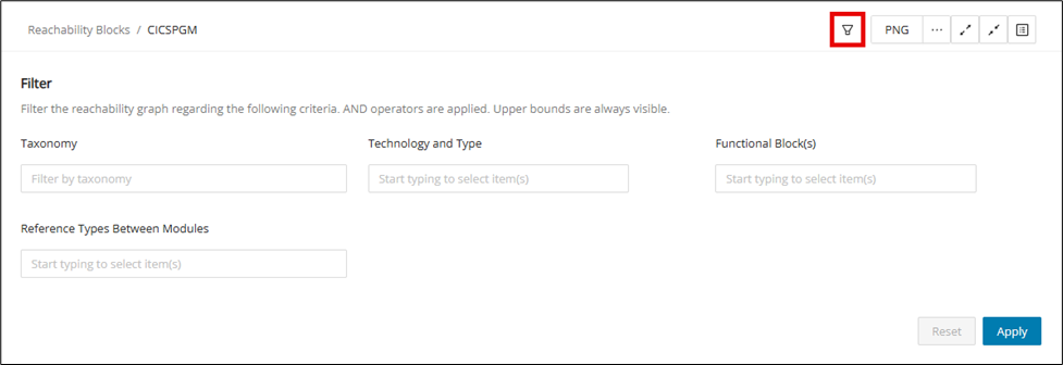
Details table
The Details Table provides a comprehensive view of how reachability blocks interact within your system, displaying detailed relationships between upper-bound and lower-bound modules. Each row captures information such as the access modules, access methods, name and technology of the upper/lower bounds. You can customize the table to your liking and adjust the level of detail by grouping data in various ways. This section will guide you through the table’s features, helping you analyze module interactions and access patterns with precision.
Open the Details Table from the Block View toolbar
To open the Details Table, select the module(s) to include in the Details Table and click Details Table .
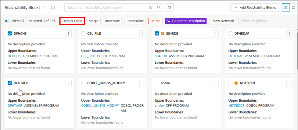
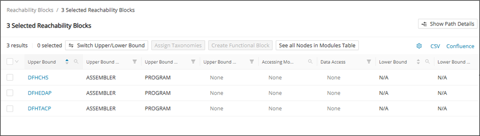
Open the Details Table from an individual block
You can also open the Details Table directly from an individual Reachability Block. Simply click the menu icon of the block and click Details Table from the drop-down menu.
Toolbar
| Button | Description |
|---|---|
| Switch Upper/Lower Bound | See all Nodes in the Modules Table |
| Assign Taxonomies | Assign Taxonomies for Upper or Lower Bound(s) |
| Create Functional Block | Ability to create a functional block by selecting one or more reachability blocks |
| Splits multiple Accessing Modules and adds intermediate modules and path taxonomies | Opens a new tab to the Modules page with a table of all of the nodes in the Details Table |
| Show Path Details | Splits multiple Accessing Modules and adds intermediate modules and path taxonomies |
Switch upper/lower bound
Info
Switch Upper/Lower Bound only appears when multiple blocks are in the Details Table.
Assign Taxonomies
Select upper/lower bound(s) and click Assign Taxonomies .

Select the Taxonomies to assign and click Save .
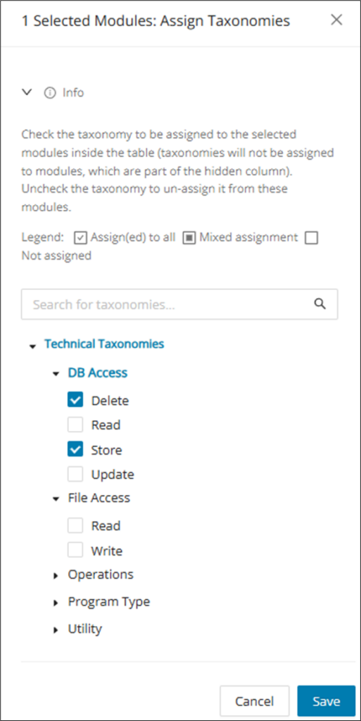
Technical taxonomies in RB Details Table and CSV
The technical taxonomies below are supported and need to have the related utility added.
| Utility | Taxonomy type | Taxonomy |
|---|---|---|
| ADUUMAIN | Operations | Unloads Table |
| ADUUMAIN | DB Access | Read |
| AMUUMAIN | Operations | Loads Table |
| AMUUMAIN | DB Access | Store |
| JZOSPROC | Operations | Runs a JAVA Program |
| NDMBATCH | Operations | Network Data Mover |
| INFOPAC | Operations | Generates Report |
Show/hide path details
Click Show Path Details to add intermediate modules. Intermediate modules are the modules that can be reached by going from the upper bound toward the lower bound (excluding the upper bound, the lower bound, and the accessing modules' names, as these are already displayed separately).
Upon clicking Show Path Details , the data in the Accessing Module column will be split into two different rows (if there are two or more access modules for the same lower bound).
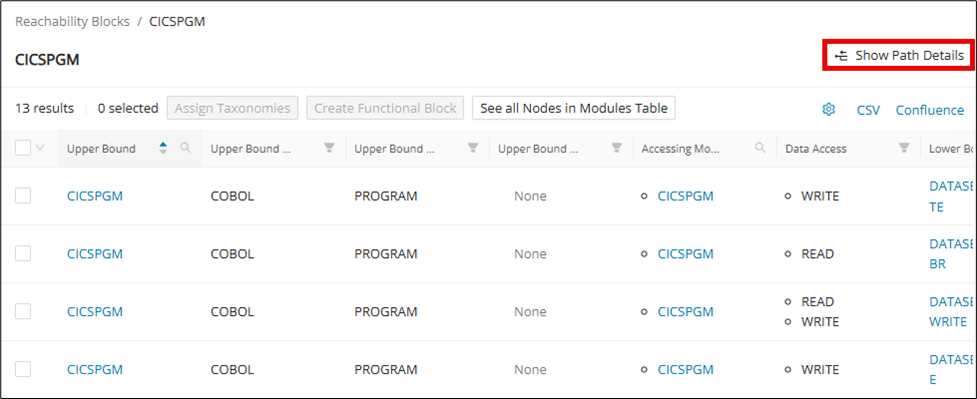
If you click Hide Path Details , the Intermediate Modules column is removed from the user interface, and the Accessing Module column is displayed again.
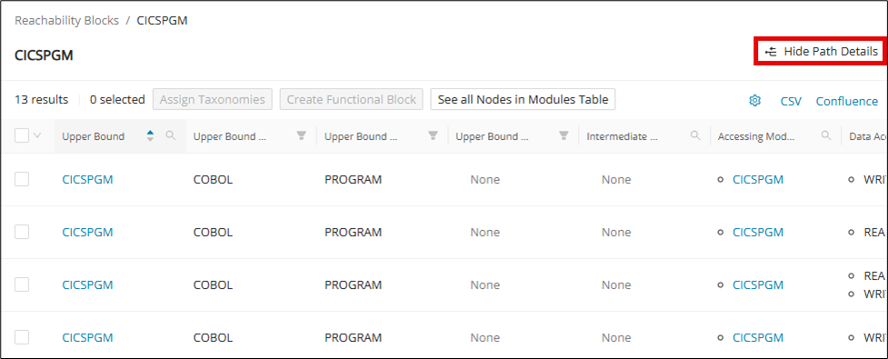
Merge
Reachability blocks can be merged to form a Merged Block. From the Block View, select two or more reachability blocks to enable the Merge button.
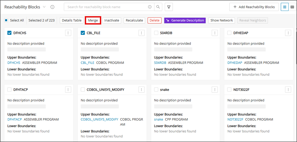
Click Merge and enter the name and description of the Merged Block. Then click Merge .
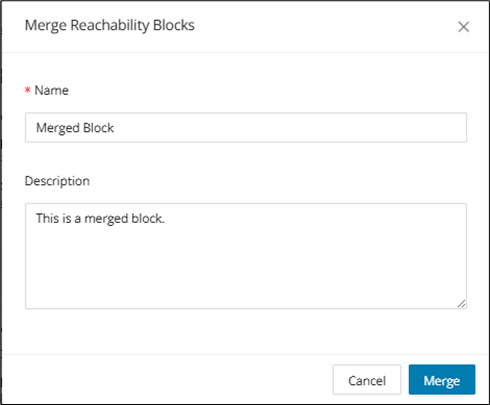
The new Merged Block is created and ready to be used for reachability analysis.
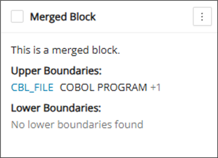
Add/remove Reachability Block(s) to a merged block
To add or remove blocks to a Merged Block, click the Merged Block to bring up its Details view. In the Details view, switch to the Blocks tab.
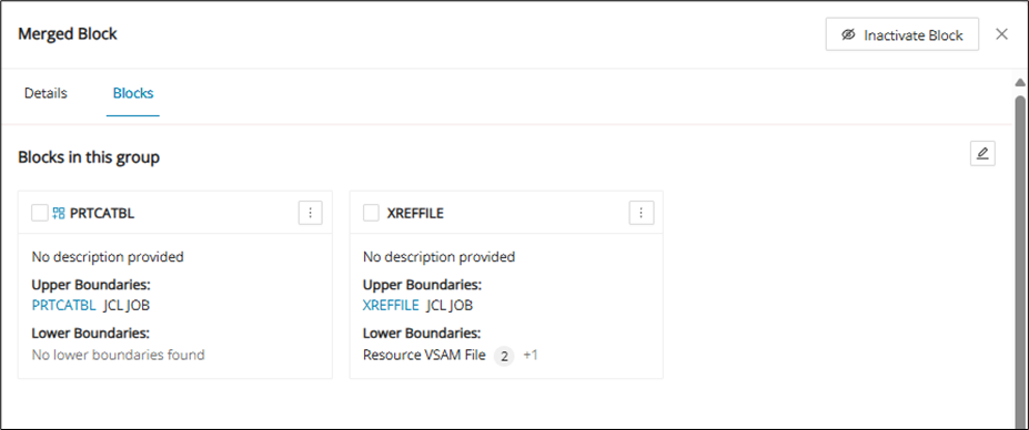
Click the edit icon for a drop-down that gives the option to either add or remove.
Add Reachability Block to merged block
Adding reachability blocks to a Merged Block shows the other reachability blocks that are not in the Merged Block. Select the desired reachability block(s) to merge into the Merged Block and click Save Updates .
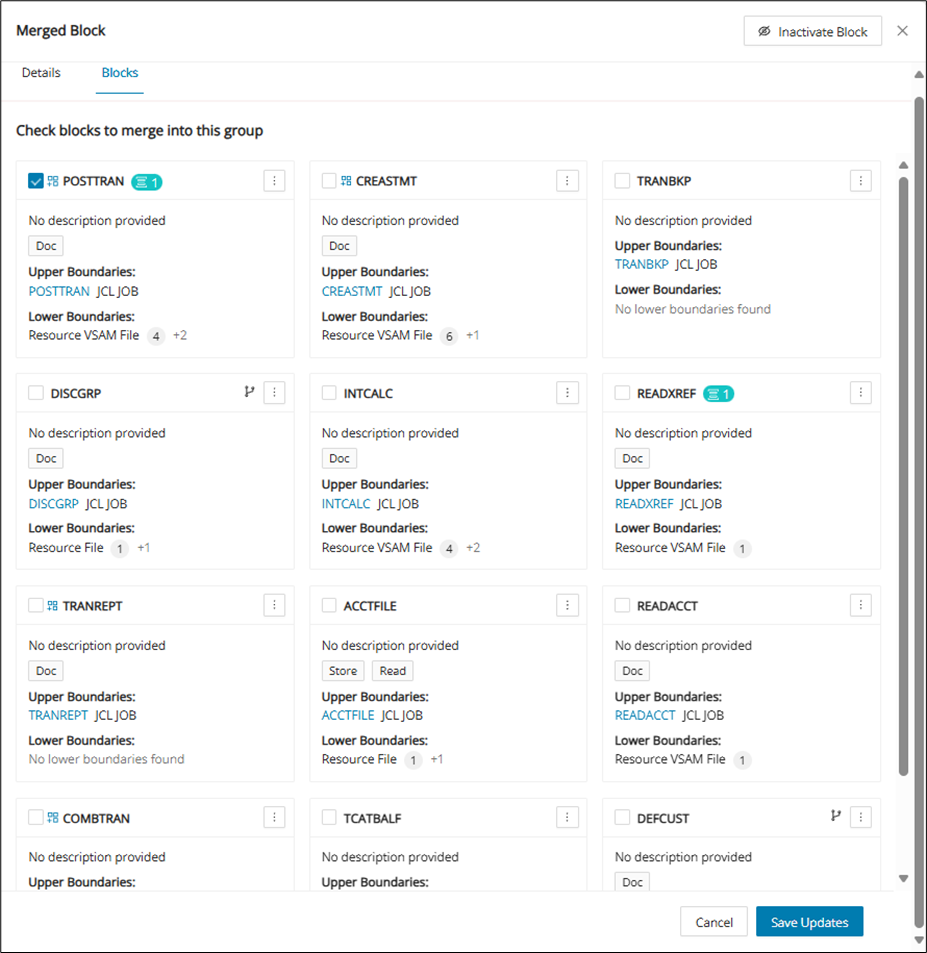
Remove Reachability Block from merged block
Removing reachability blocks from a Merged Block shows the reachability blocks that are within the Merged Block. Select the desired reachability block(s) to unmerge from the Merged Block and click Save Updates .
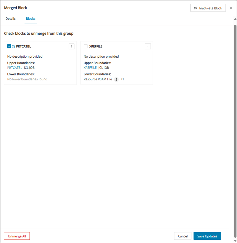
Unmerge all
To simply unmerge all reachability blocks within a Merged Block, click Unmerge All at the bottom of the Block tab in the Merged Block's Details view.
Inactivate
Reachability blocks can be inactivated to be hidden from all views unless explicitly activated. To inactivate a block from the Block View, select the reachability block(s) to inactivate and click Inactivate .
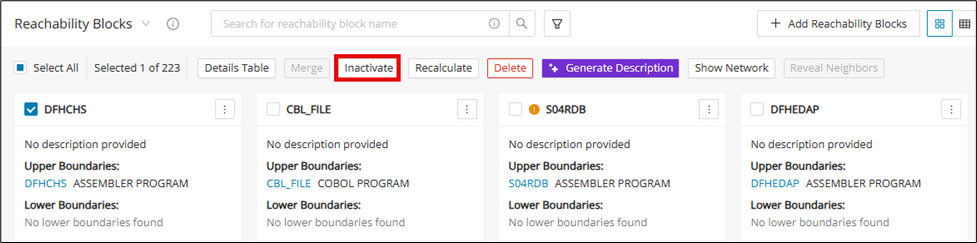
An individual reachability block can also be inactivated from its Details view. Open the Details view and click Inactivate .
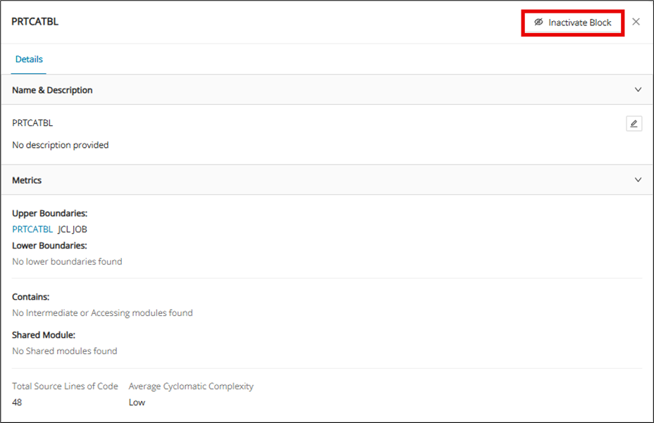
To show inactive blocks, click the filter and toggle on "Show inactive blocks".
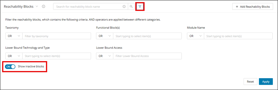
Inactive blocks are marked as "Inactive" at the top of the block.
Re-activate block
To re-activate a reachability block, make sure the "Show inactive blocks" toggle is on inside the filter. Click an inactive block to open its Details view and click Activate Block .
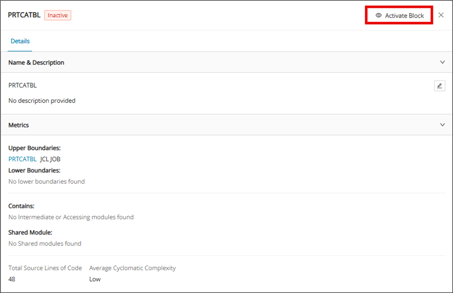
Recalculate
When reachability blocks need to be updated, they can be recalculated. Recalculation runs the selected blocks through the call chain again to make sure all updates are applied. If there were no changes in the modules or the implementation of reachability analysis, recalculation should have no effect and leave the reachability block as-is. Outdated and removed reachability blocks cannot be recalculated.
Recalculation for individual block
Click the menu icon of the block to be recalculated and then click Recalculate from the drop-down.
Recalculation for multiple blocks
Select the reachability block(s) on the Block View and then click Recalculate .
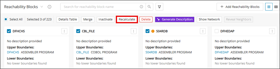
Recalculation in network view
Select any block in network view and click the recalculate icon.
Delete
In the Reachability Blocks page, you can delete a reachability block by selecting the upper-left corner box and clicking Delete . Only users with the key cloak role: Admin, Client-Admin, and Manager have the permission to delete Reachability blocks.
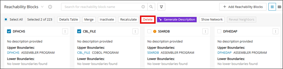
A pop-up warning is displayed when deleting a reachability block(s). Click Delete to confirm the action.
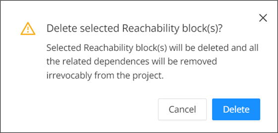
Generate description
Navigate to the Reachability Blocks overview screen, select a few reachability blocks, and click Generate Description .
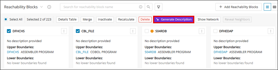
Module descriptions should be available for the modules available in reachability blocks while generating descriptions using Gen AI. If description is not present, then generate missing module descriptions checkbox should be checked.
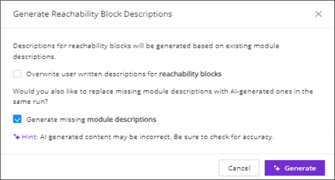
To override any reachability block description, check the "Overwrite user-written descriptions for reachability blocks" checkbox while generating using Gen AI.
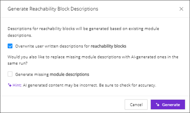
Click Generate to generate the reachability blocks description.
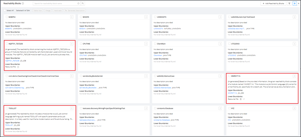
Descriptions can be seen in the reachability overview screen as well as in the view details.
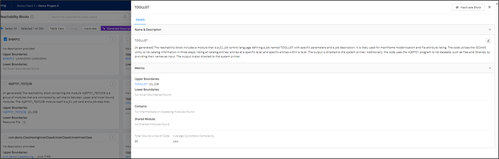
Show network
A reachability network is a dependency graph, illustrating connections between all reachability blocks via shared lower bounds. The direction of the arrows indicates a producer-consumer relationship, that is, a producer block writes into a shared lower bound, which is then consumed or read by the consumer block. A bi-directional connection means both of the blocks are either producers, consumers or both.
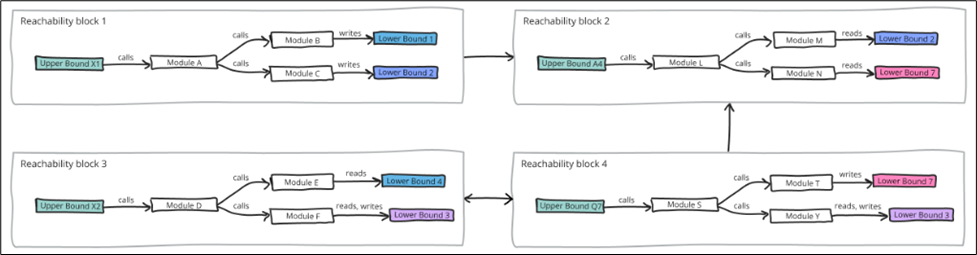
Furthermore, you can also see the actual job dependencies between the blocks by importing scheduler data under Configuration.

Show predecessor/successor
After creating reachability blocks, it is possible to display their reachability network by clicking the Show Network drop-down menu. From here, the options to Show predecessor and Show successor are available.
- Predecessors are blocks that provide data to the selected block. In the diagram below, Blocks A and B are predecessors of Block C, as the data produced by these 2 blocks is used by Block C to write to its own lower bound.
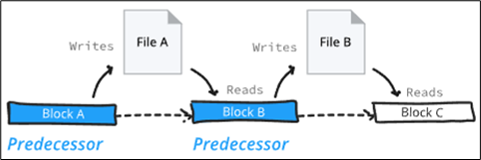
- Successors are blocks that receive data from the selected block. In the diagram below, Blocks B and C are successors of Block A, as the data produced by Block A is consumed by Block B and further by Block C to update or write into their own lower bounds.
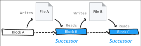
Click Show predecessor or Show successor to provide the network view of the selected blocks.
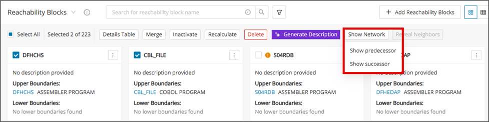
After clicking Show predecessor or Show successor , a pop-up window related to the selected reachability blocks will be shown. Each row represents a lower bound of the selected reachability block, and when selected, it will be included in the network view shown. At the bottom of the window, select the specific file types of the lower bounds to further narrow down the network view. Select the lower bounds and click Proceed to produce the network view.
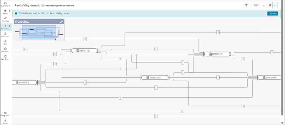
Network View offers similar functionalities to Block View. Four buttons will be shown by clicking each reachability block:
| Icon | Description |
|---|---|
| View Details: opens the details panel for the selected reachability block. | |
| Details Table: opens the Details Table for the selected reachability block. | |
| Details Graph: displays the graphical representation of how each modules are connected within the selected reachability block. | |
| Recalculate: reruns the call chain to update the reachability block |
Reachability Blocks network view
The Reachability Blocks Network View provides access to the complete network view of the connections of all the reachability blocks. To access this view, you must enable the reachabilityResourceNetwork feature toggle, which replaces the Show Network button with a dedicated Network View icon in the top right corner of the interface.
Configuration
To use this feature the reachabilityResourceNetwork feature toggle must be enabled.
From the Block View, navigate to the page header and click the Network View icon to switch between the block and network view.

If two reachability blocks share the same lower bound, then they will be linked in the network.
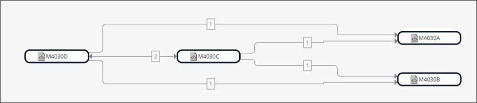
Otherwise, reachability blocks that do not share a lower bound will not be connected in the network view. Blocks without any connections can even be isolated, like in the picture below.
Merge blocks from Network View
Multiple Reachability Blocks can be selected and then merged, similar to the Merge feature in the Block View.
Select two or more nodes in the network view using Ctrl+Click (on Windows) or Cmd+Click (on Mac). Then click on the Merge icon.
Info
The Merge icon will only be displayed when selecting two or more nodes.
Step 3:
A Merge Reachability Blocks dialog is displayed. Enter the block name and description and click Merge. Once merged, the network is recalculated, and the links are rearranged with respect to the merged block.
Reachability Network View filters
This function allows you to filter out reachability blocks and their edges in the reachability network to view the most important information needed for analysis.
The reachability network view window displays filters for:
Edge filtering:
Shared lower bound technology and type filter:
Filter modules by technology and type of the shared lower bound. For example, if you enter either a technology or a type of the shared lower bound, all possible technology-type combinations of the supported lower bound will be shown so that you can select the most suitable combination.
Values for the dropdown:
Populate the lower bound technology and type values for all existing reachability blocks in the screen. If a new reachability block gets created with a new lower bound technology and type, this list will grow and show the new technology and type for the newly created reachability block.
Multiple options can be selected from the filter drop-down lists.
Step 1:
Click the filter icon.

The reachability network view displays all of the filter options.
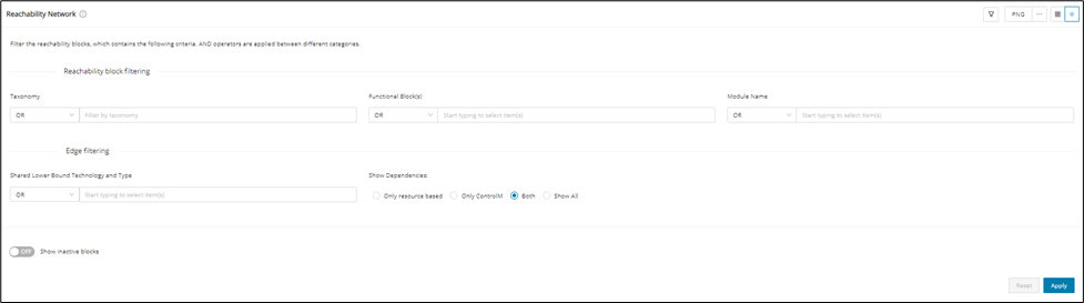
Step 2:
Filter Shared Lower Bound Technology and Type as "Resource File".
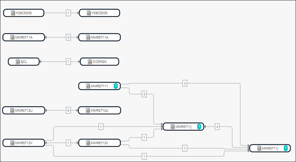
Reveal neighbors
The “Reveal Neighbors” feature provides miners with hints about unrevealed blocks that are not immediately visible during the initial analysis due to predefined criteria. This ensures miners can access crucial information in neighboring blocks, leading to a more comprehensive understanding of the blockchain structure.
Info
Note that the icon, which, when hovered, indicates if a block contains hidden neighbors.
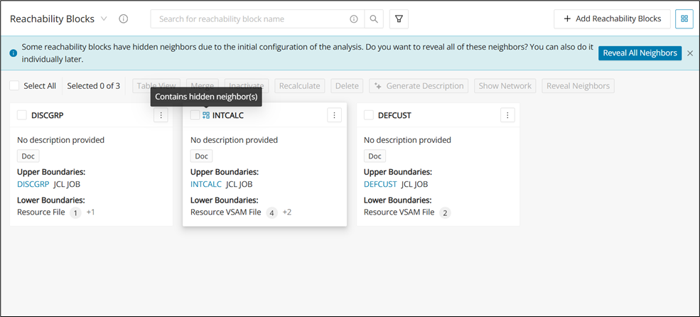
Select at least one block with undiscovered neighbors and then click Reveal Neighbors.
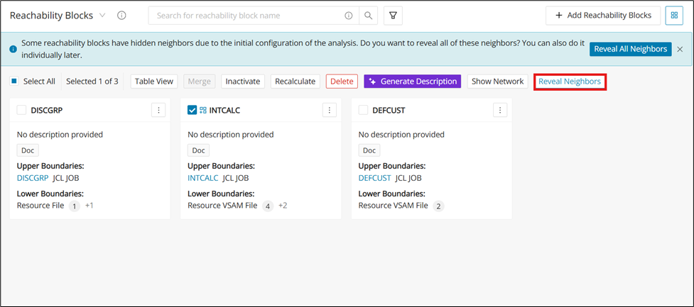
Or just click Reveal All Neighbors located on the banner at the top, which will act on all blocks with hidden neighbors.
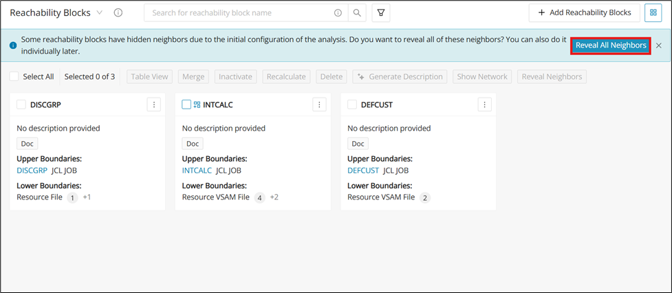
You can also reveal neighbors from the Network View.
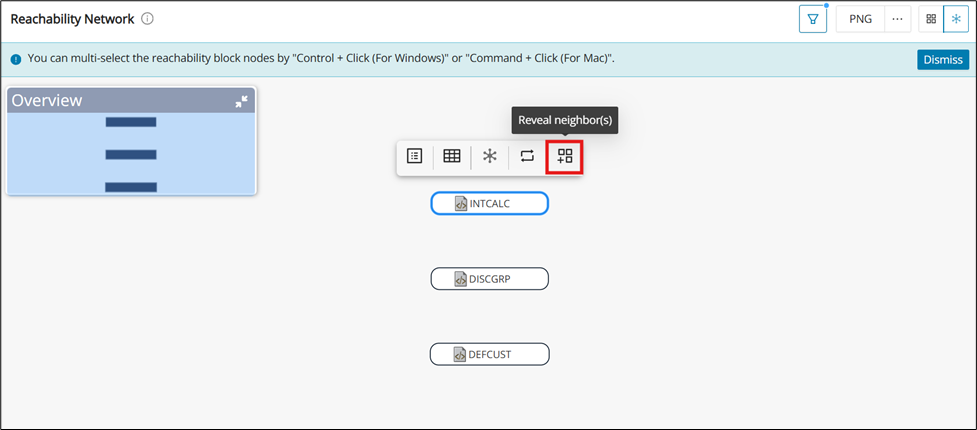
Examples
The following examples show how reachability features are applied in common analysis scenarios. Use them to understand how the overview, details table, and taxonomy actions work together in practice. Each example focuses on a concrete workflow you can reproduce in the UI.
Taxonomy assignment in Reachability Block(s) based on upper bound taxonomy
For a single reachability block in a Details Table, an option is provided to choose and apply the upper bound taxonomy to the lower bound modules, as well as all the underlying modules in the call chain, based on the Intermediate module details and whether the lower bound module is a read edge or a write edge module.
Step 1:
Navigate to the Reachability Blocks overview and find the desired reachability block. Check Select All and then click Details Table to populate the upper and lower bound taxonomies.
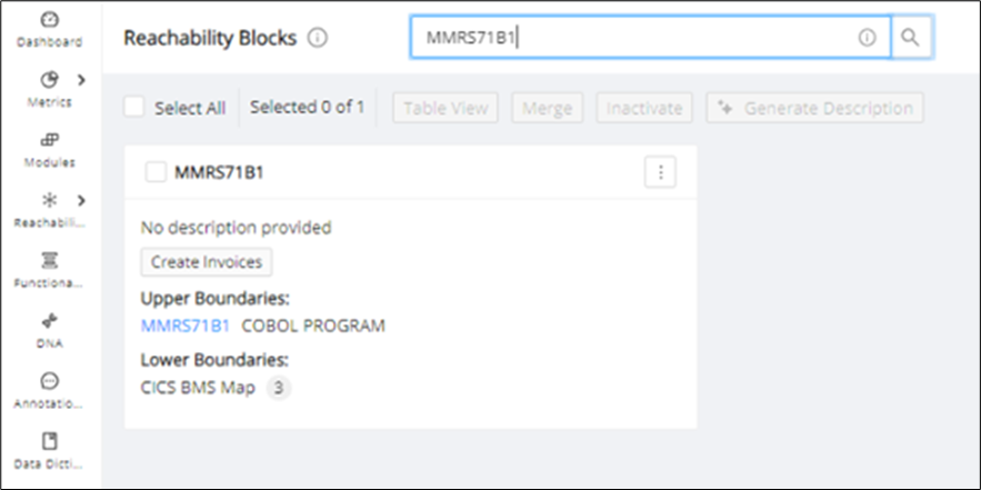
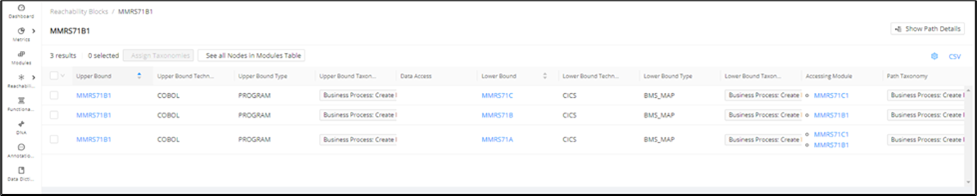
Step 2:
After clicking the select box of the desired reachability block, the Assign Taxonomies button will be enabled. Click Assign Taxonomies .
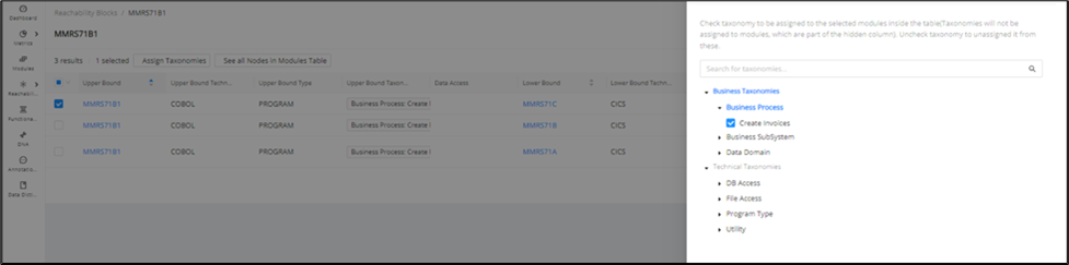
Step 3:
After assigning the taxonomies, they will be applied to all modules selected in the table row.


Step 4:
Changes to the taxonomies will also be reflected on the module details page and search for the modules.
Click CSV to download the CSV file. The updated taxonomies will be available in the CSV export in the Lower and Upper bound taxonomy columns.

Reachability Block datapoint in Modules table
Filter modules by reachability block to display the modules that are included in the reachability block.
Step 1:
Navigate to the Modules page, click the settings icon, search for “Reachability Block Name”, and select the checkbox. A new column will then be added to the table.
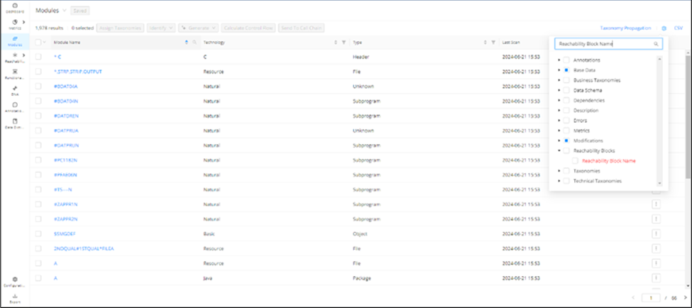
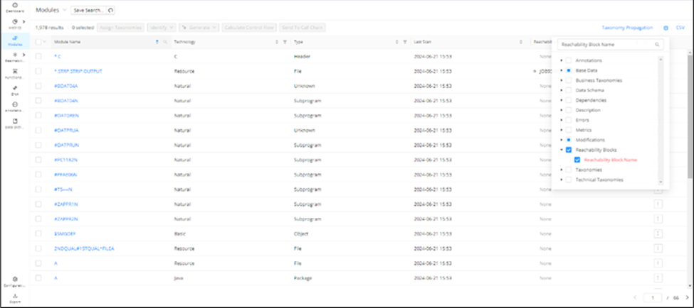
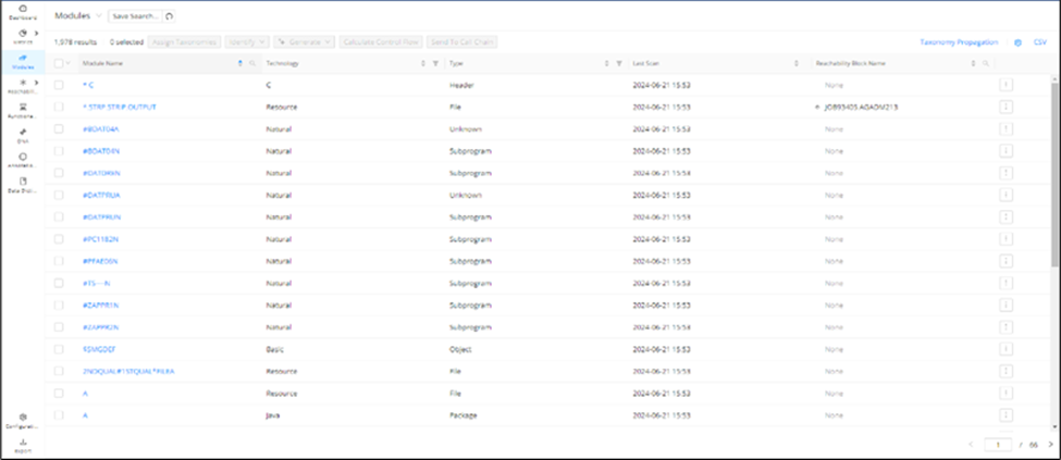
Step 2:
Click the search icon in the “Reachability Block Name” column. The info icon is present in the search field with a tooltip shown below. The user can search reachability blocks with either the full name or with wildcards.
The reachability block names will appear in alphabetical order as a list in case there is more than one reachability block name appearing per cell.
Shared lower bound information
A Shared Lower Boundary is when two reachability blocks have both read and write access to the same lower boundary. In the network view of the reachability blocks, you can see the shared lower bound information on the edge linking the two reachability blocks.
The number on the edge indicates how many lower bounds are being shared between the two reachability blocks. This number is clickable and will indicate the number of common lower bounds when it is hovered over.

Clicking the number opens the "Common Lower Bound(s) Details" dialog on the right side of the screen.
Next to the "Common Lower Bound(s) Details," there is an info icon. Hovering over it shows a pop-up with information about shared lower boundaries.
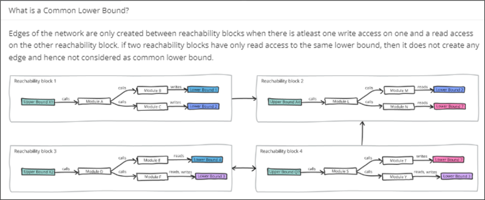
Shared lower boundaries are visible and are collapsed by default. The name of the shared lower boundary is visible as a header. When expanded, the following information is displayed:
-
Technology
-
Type
-
Access Types
-
Taxonomies
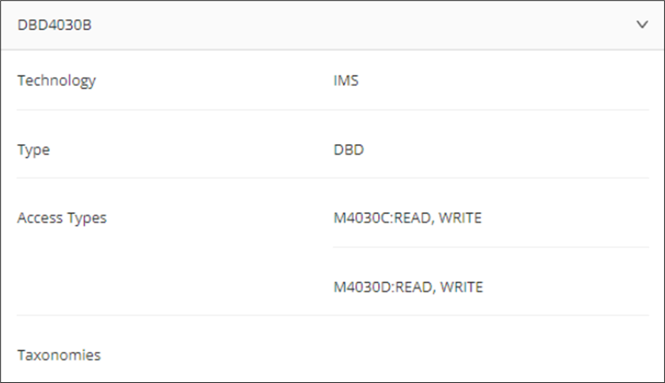
In the Access Types section, it shows that both reachability blocks have read and write access to the shared lower boundary. The same information about the shared lower boundary and block access types is available in the reachability block Details Table.
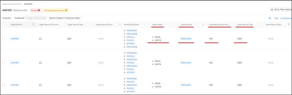
Upper/lower bound taxonomies in the Details Table
The Details Table features are as follows:
- The Detail Table displays all information for the reachability block(s), even if no lower bound modules are present.
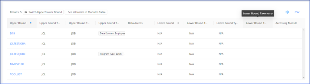
-
All taxonomies assigned to the upper and lower bound modules can be viewed along with their respective taxonomy terms in two separate columns:
-
Upper Bound Taxonomy
-
Lower Bound Taxonomy
-
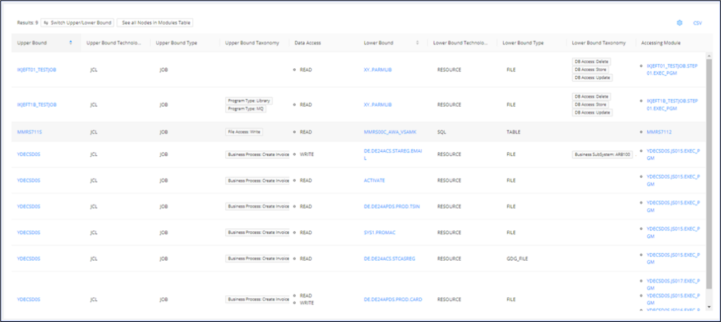
- To export the table, click CSV in the top right corner of the table.
-
The export will download as a CSV file named reachabilityData.
-
The CSV file contains the same taxonomies in the respective columns as they are displayed in the UI Details Table.

Filter for taxonomy columns in the Reachability Block Details Table screen
Navigate to the Reachability Blocks overview and find the desired reachability block. Select all of the blocks then click Details Table to populate the upper and lower bound taxonomies. Click the settings icon and select Path Taxonomy to view Path taxonomies.
The following columns have filter and reset capabilities when clicking the filter icon next to the column name:
-
Upper Bound Name
-
Upper Bound Technology
-
Upper Bound Type
-
Intermediate Module Name
-
Accessing Module Name
-
Data Access
-
Lower Bound Name
-
Lower Bound Technology
-
Lower Bound Type
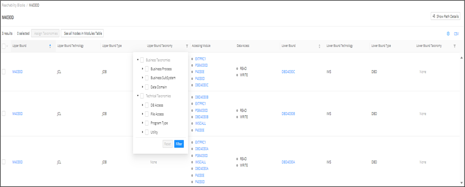
Info
The columns that support wildcard search are: Upper Bound Name, Lower Bound Name, Intermediate Module Name, Accessing Module Name.
The Upper Bound Technology, Upper Bound Type, Lower Bound Technology, and Lower Bound Type columns have a multiple-choice filter that lists all of the technologies and Types present in the column of the reachability block.
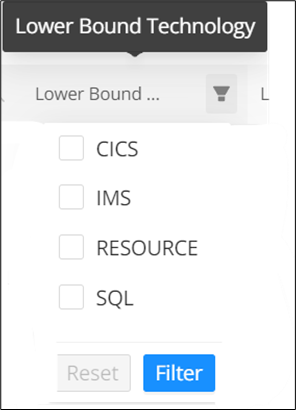
The filter for "Data Access" gives the list of all data accesses present in the column.
Functional Analysis
Functional blocks help you to represent business logic and are made of code annotations to form larger functional structures across one or more modules. Review the Modules page for the multiple ways that annotations can be created or generated. Once created, you can see them in a control flow graphical view (technical annotation level) or process flow graphical view (abstracted functional block level).
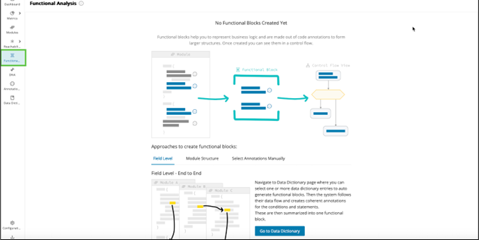
Role-based access control (RBAC)
This section contains information on role-based access control for editing functional blocks. Access control on functional block screens is based on three user roles:
-
Viewer: Can only view the functional blocks/groups and does not have permission to create, edit, delete, or rename the existing functional blocks/groups.
-
Editor: Can create, edit, modify, and delete the Functional Blocks, but cannot perform any bulk operations. For example, bulk deletion of functional blocks.
-
Manager: Can create, edit, modify, delete, and perform bulk operations.
| Operation | Viewer | Editor | Manager |
|---|---|---|---|
| Filtering on the Functional Analysis landing page | Yes | Yes | Yes |
| Group/ungroup functional blocks | No | Yes | Yes |
| View functional blocks in tree view | Yes | Yes | Yes |
| Expand/collapse functional block in tree view | Yes | Yes | Yes |
| Select and view functional block or annotation details in the tree view | Yes | Yes | Yes |
| Click the modules and navigate to the module detail page | Yes | Yes | Yes |
Functional Blocks creation
Functional Blocks provide great flexibility in how they allow grouping code together. Mining supports several creation paths so you can choose the one that best matches your analysis goal and available metadata. The options below summarize the main ways to create or generate functional blocks.
Manual Functional Block creation
Manual Functional Block Creation starts in the Code Viewer while reviewing the annotations within a module. Once an annotation is created, you can click on its Functional Block icon as the starting point to create and define a Functional Block. For more detail read through the Functional Block tab under Managing Annotations in Code Viewer
Reachability Analysis (E2E flow)
When the Reachability Analysis has been conducted on your project. You can leverage its generated end-to-end (upper bounds to lower bounds) process flow results to generate functional analysis along any or all of its flows as well. This enables you to quickly drill down one level and begin to extract the business logic within the individual modules after decomposing your application at the highest level.
Step 1:
On the Reachability Analysis Block View page, select your reachability block of interest and click Details Table button in the toolbar.
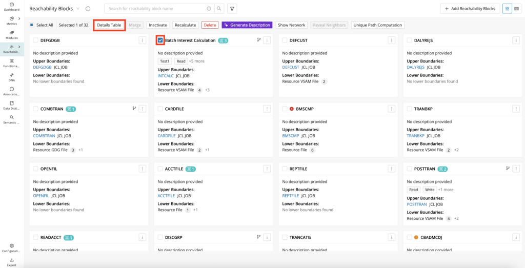
Step 2:
From the Details Table, select each of the E2E flows inside your selected reachability block that you would like to capture functional analysis for, and click Create Functional Block in the toolbar. A confirmation modal will appear next, where you can click Create Functional Block to generate the Functional Blocks.
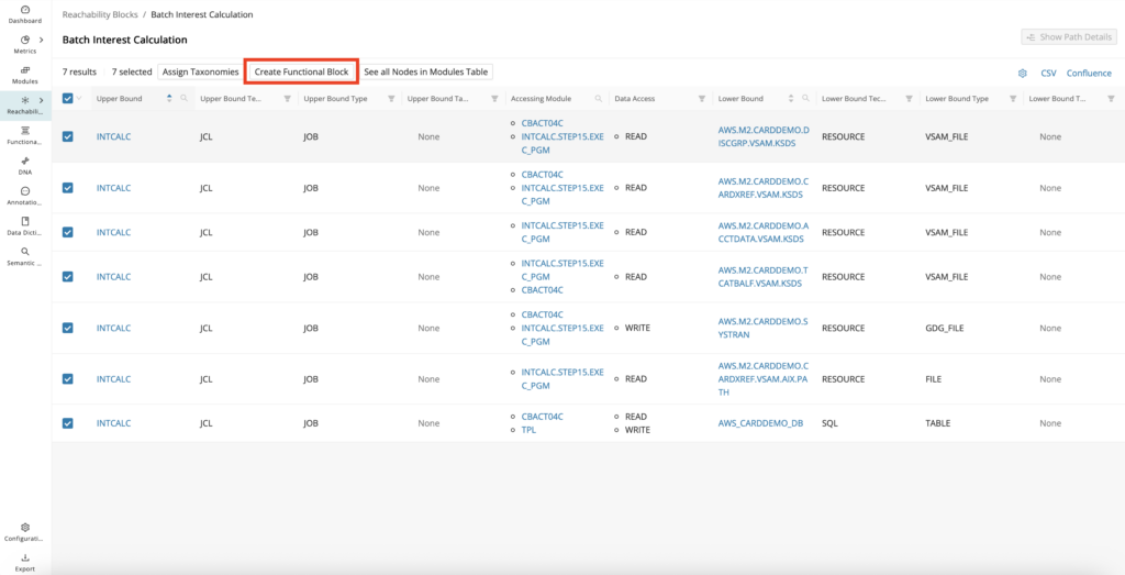
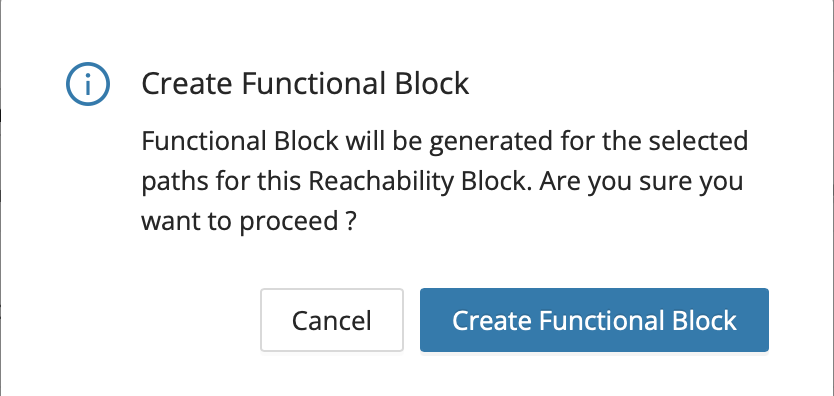
Step 3:
To view the output, click on the Functional Analysis menu option on the far left menu pane. The generated Functional Block(s) will be shown in the tree view of the Functional Analysis page.
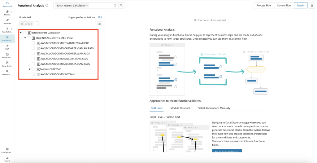
Module structure
Functional Blocks will be generated per the skeletal outline of the program, grouping annotations within this structure, or even if they are empty (for example, if no Annotations exist). Functional Blocks generated per the module structure allow a quick functional overview of the entire program from top to bottom, and if present, to see the annotated business logic within that structure.
Info
Enable the feature toggles structuralFunctionalGroups to create Functional Blocks per the Module structure without existing annotations.

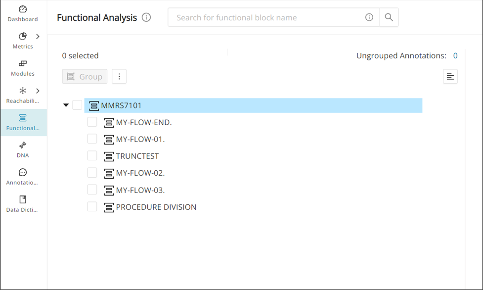
The application generates the functional block when you select a supported module and click Identify Functional Block from the drop-down menu.
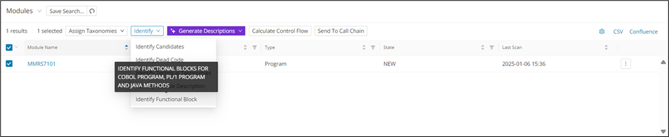
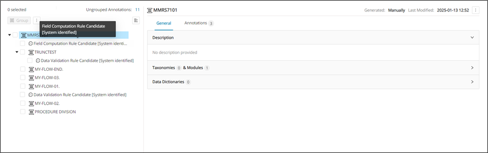
In the figure above, you can see the Functional group containing “Functional units” on the left-hand side. If you click Control Flow at the top right, you will see a filtered control flow graph.
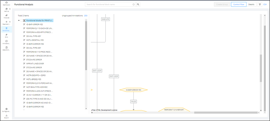
Similarly, if any conditions are present between annotated statements and the entry point for the conditions, functional conditions are created.
Java Functional Blocks
Functional Analysis supports the generation of automated Functional Blocks for Java, where Functional Blocks are created per Java methods along their Call Chain. The detail view, which is displayed next to the blocks, shows the Java methods and classifies the annotation type as FUNCTIONAL, category as none, and state as CANDIDATE. For more info on the details view, refer to the Details View for Functional Analysis
Info
For Java methods, the feature toggle javaCollectMethodCalls must be enabled before Code Discovery; otherwise, it will not generate, and Java methods will show as unsupported.

Field Level Mining
Unlike auto-generated Functional Blocks based on Module Structure, with Field Level Mining generated Functional Blocks contain all the annotated statements along a data flow path across modules stemming from a selected field. It uses Data Lineage to capture this flow and create the Functional Blocks. This allows miners to zoom in on the business logic associated with each selected field to better understand its impact and plan/implement the modernized system.
Field Level Mining can be conducted from the CodeViewer on individual fields if you prefer to see the source code, or from the Data Dictionary in bulk if you know the fields of interest upfront.
Conducting Field-Level Mining from the CodeViewer
Step 1:
Open the CodeViewer, right-click on the field of interest, and select Identify Functional Block.
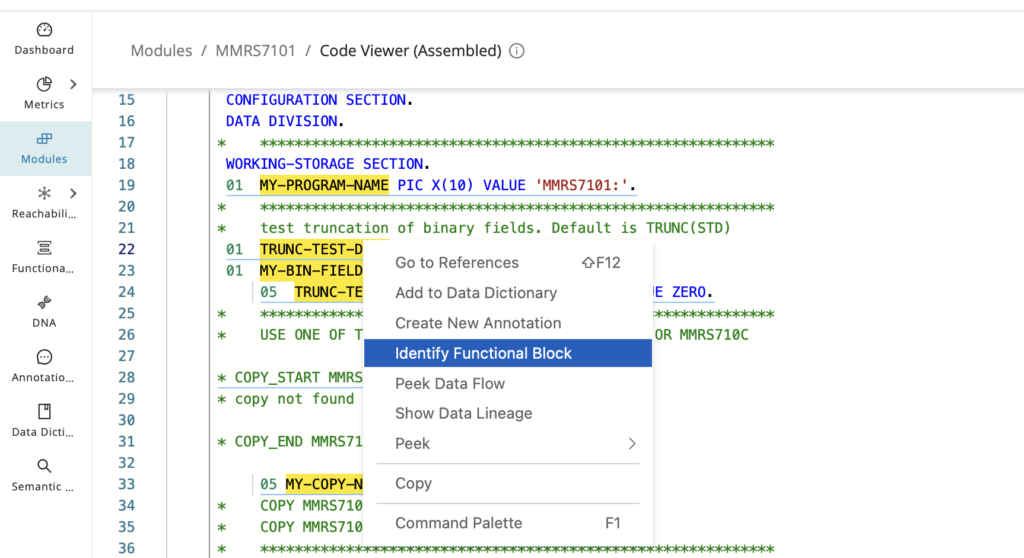
Step 2:
To view the Field Level Mining output, click on the Functional Analysis menu option on the far left menu pane. The generated Functional Block(s) will be shown in the tree view of the Functional Analysis page.
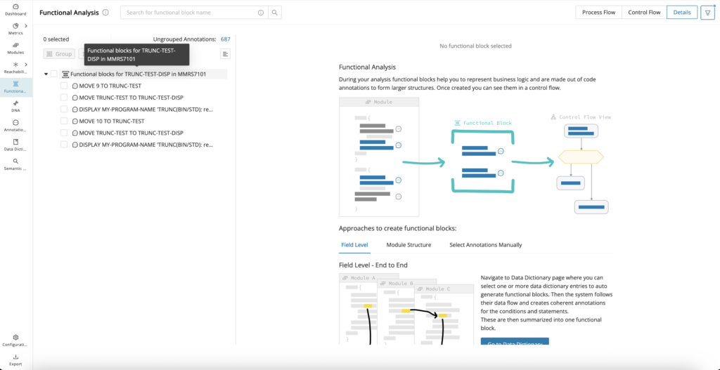
Conducting Field Level Mining from the Data Dictionary
Step 1:
You can search Data Dictionary Entries across your project (Data Dictionary Reporting page) or at a single module level (Module Detail Page - Data Dictionary tab). From either of the Data Dictionary tables, select one or more fields of interest, and select Identify Functional Block.
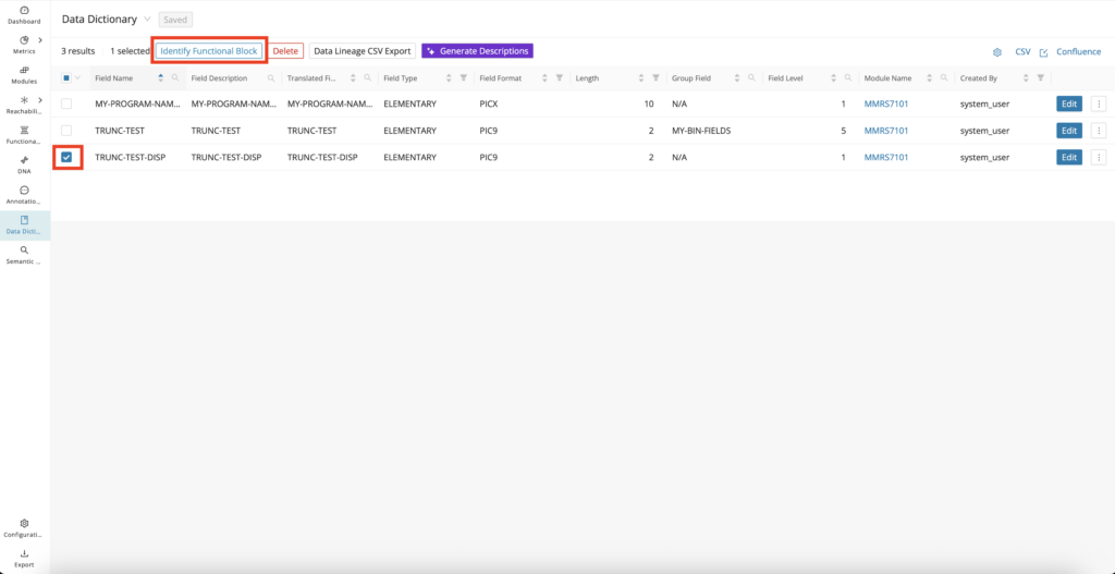
Step 2:
To view the Field Level Mining output, click on the Functional Analysis menu option on the far left menu pane. The generated Functional Block(s) will be shown in the tree view of the Functional Analysis page.
Semantic Functional Block
Uses GenAI capability to group similar code within a module into Functional Blocks, which are also given meaningful names and descriptions.
Info
Enable the feature toggle semanticFunctionalBlockGeneration.
Step 1:
From the Modules Reporting page, select one or more supported modules of interest, click Identify from the toolbar, and select Generate Semantic Functional Block from the drop-down.
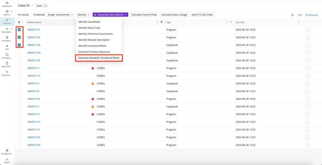
Step 2:
There is an option to configure how many annotations are captured inside the Functional Blocks, along with a similarity threshold if needed. Otherwise, click Submit with the set default values to generate the Semantic Functional Block(s).
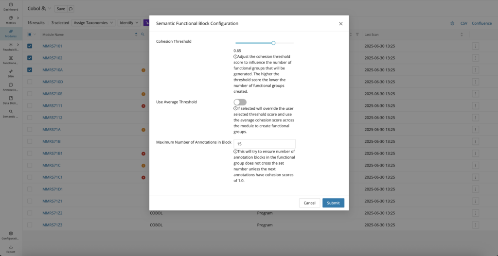
Step 3:
To view the Semantic Functional Block output, click on the Functional Analysis menu option on the far left menu pane. The generated Functional Block(s) will be shown in the tree view of the Functional Analysis page.
Filtering and sorting Annotations by Functional Blocks
To view functional blocks on the Annotations tables:
Step 1:
Click the settings icon on the top right corner and select Functional Blocks > Functional Block Name.
Step 2:
Click the up and down arrows on the Functional Block Column header to sort the content.
Step 3:
Search for a specific functional block name using the search icon.
Modules associated with the searched functional block will now be displayed.

Functional Block analysis results
After creating functional blocks, the Functional Analysis is automatically populated with a Tree View to the left and a Details View on the right. From here, you can view and edit the functional block structures and even see these functional blocks in a control flow view or process flow view.
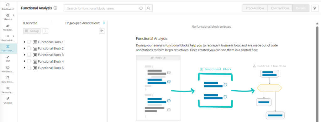
Tree view
The Tree View in the Functional Analysis page allows you to easily organize and rearrange functional blocks and annotations by simply dragging and dropping them across functional blocks.
Select the annotation or functional block that needs to be moved and drag and drop it into the desired functional block. If the order must be rearranged, drag the annotation or functional block to the desired spot. Dragging and hovering over a non-empty functional block will auto-expand the block to enable this ordering operation. This auto-expansion applies to non-empty sub-functional blocks as well.
Dragging an annotation or functional block outside of the tree (above the first functional block) will display an error message

Group/Ungroup
Grouping Functional Blocks
You can group functional blocks or annotations from the Functional Analysis page.
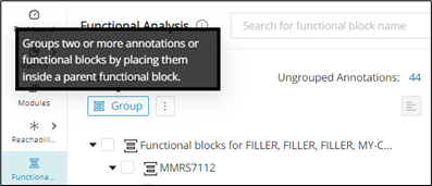
Select 2 or more functional block(s) at the same level and click Group .
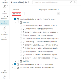
Or select 2 or more annotations at the same level and the same part of the functional block and click Group.
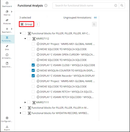
Warning
Group cannot be used when the selected functional blocks and annotations are not appropriately at the same level.
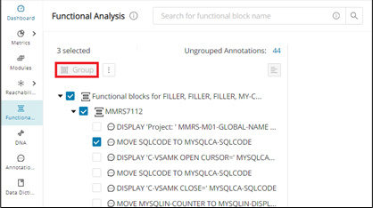
Splitting automatic Functional Blocks
You can modify automatically generated functional blocks to split annotations within a large functional block into a smaller functional block. The CFG of the large functional block will then display the smaller functional block as a collapsible group containing the selected annotations.
Step 1:
Navigate to the functional analysis page and expand any auto-generated functional block and select the annotations to be put into a smaller functional block, and click Create Group .
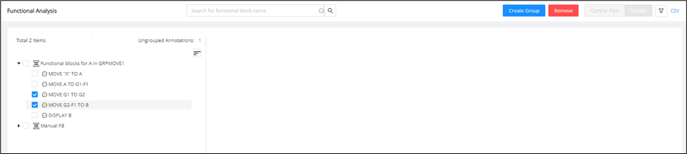
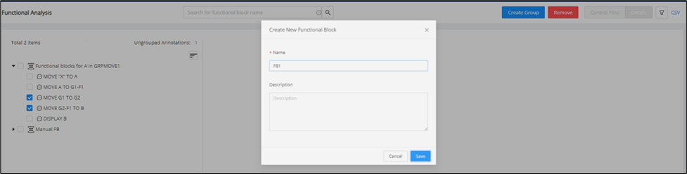
Step 2:
Once the new blocks are created, the selected annotations will split into their own new functional block. The new group will be created as the last child item.
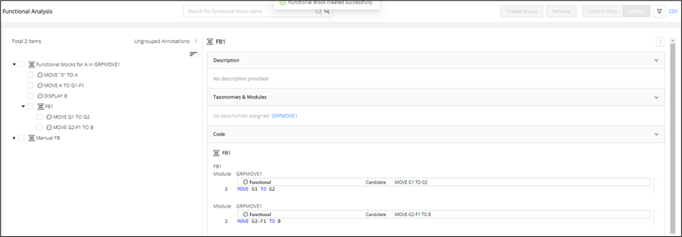
Step 3:
Click the Functional Block and click Control Flow , which will display the smaller functional block as a collapsible group in the CFG.
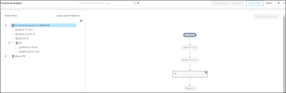
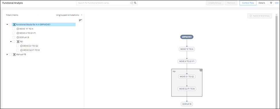
Ungrouping Functional Blocks
You can ungroup non-empty functional blocks on the functional analysis page. When ungrouping a functional block, the group functional block will be removed, and the assigned annotations will be unassigned. Any child of the formerly grouped functional block will go one level above.
Navigate to the Functional Analysis page and select the non-empty functional block(s). Click the menu icon next to "Group" to display the Ungroup button from a dropdown menu. Click +""Ungroup"++ to Ungroup the selected non-empty functional block(s).
Warning
Selecting annotations or a mix of annotations and functional blocks will deactivate the Ungroup button.
Functional Block grouping hierarchy
The grouping of Functional Blocks will maintain its hierarchy in the Functional Analysis page.
Grouping Functional Blocks:
-
When you select two functional blocks (block1 and block2) and then click Create Group in the Functional Analysis page, a new group (group1) will be created with block1 and block2 as its children.
-
The newly created group (group1) will be displayed correctly in the hierarchy.
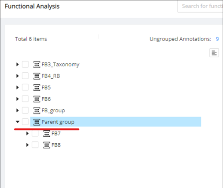
Ungrouping Functional Blocks will function similarly to an undo action. The ungrouping behavior can be revised as follows:
In the functional analysis page, if we have a hierarchy like below.
Select group2 on clicking ungroup, the system should delete 'group2'. The child functional blocks of 'group2' (for example, 'fb3' and 'fb4') should then be reassigned to the immediate parent of 'group2', which in this case is 'group1'.
Nested grouping:
-
When you expand group1, select block1 and block2 (children of group1), and then click Create Group again, a new group will be created inside group1.
-
The newly created group will maintain the hierarchy and be displayed as a child of group1.
Hierarchy maintenance:
-
The hierarchy of functional blocks will be maintained correctly when creating nested groups.
-
The parent-child relationships will be preserved, and the newly created groups will be displayed within their respective parent groups.
Generate Functional Block name and description
Configuration
The feature toggle generativeAiTranslations must be enabled in the WebUI feature console.
Quickly generate a more meaningful functional block name and/or description by using the "Generate" function, which uses Gen AI to generate content. Information from the related Data Dictionaries will be considered in the AI-generated content, and it is advised to always check for accuracy.
Click the checkbox(es) of the functional block(s) that need a description and/or a more meaningful name. Then, click the menu icon next to the Group button and click Generate Functional Block Description .
The "Generate Functional Block Description" modal will display, and you can generate the Functional Block names and/or descriptions by clicking Generate . If the selected functional blocks have existing descriptions, they can be overwritten by checking the "Overwrite existing descriptions" option.
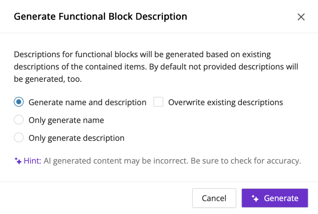
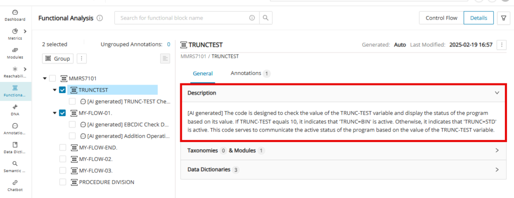
Generate Process Sequence
For the annotations encapsulated within the listed Functional Blocks, you can generate a process sequence (per the execution flow) for them across modules linked to the selected functional blocks in the tree view. This removes the need to manually analyze and sequence annotated rules using custom properties. Alternatively, you can also trigger automated process sequence generation at the module level in batch from the Modules workflow.
Info
Annotations should already exist on the modules associated with the selected functional blocks to allow the system to sequence them per their executable flow.
Click the checkbox(es) of the functional block(s) that contain annotations that need automated process sequence generation. Then click the menu icon next to the Group button and click Generate Process Sequence .
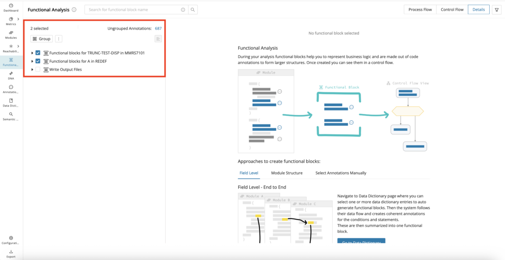
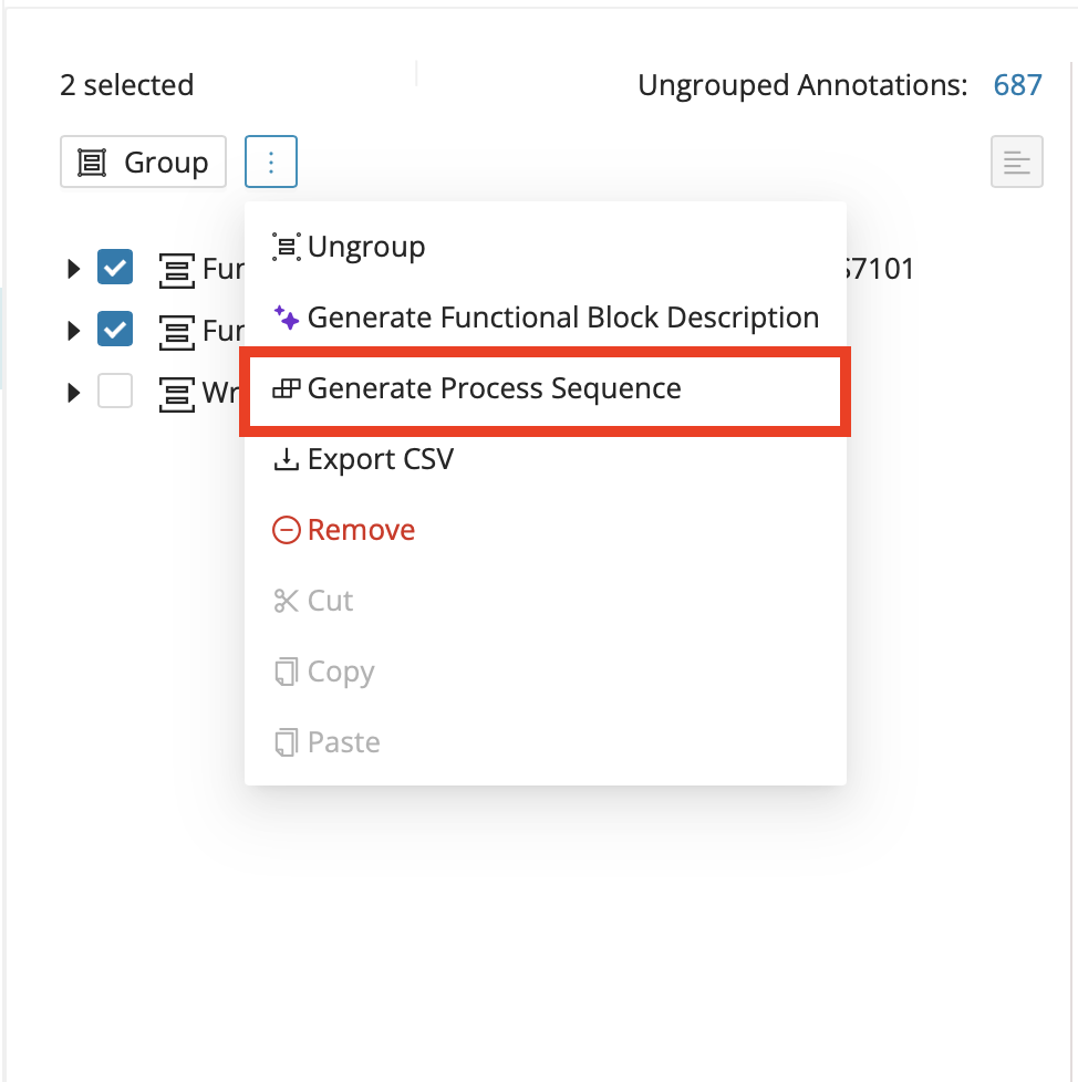
Export CSV
You can export the tree view of functional blocks as a CSV from the Functional Analysis page.
Select the functional block(s) that need to be exported and click the menu icon next to the Group button. Then click Export CSV .
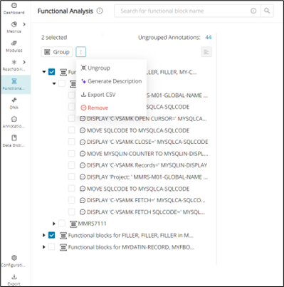
Info
The Export CSV button is still able to be used when selecting nothing to download; contents are downloaded only for the functional blocks that are available based on the filter being applied on the page.
Configuration
Selecting annotations or a mix of annotations and functional blocks will deactivate the Ungroup button.
A CSV file named functional_block_analysis is downloaded. It contains the data of the functional blocks in the sequence specified below:
-
Functional Block Sequence (Level 1)
-
Functional Block Name (Level 1)
-
Functional Block Description (Level 1)
-
Functional Block Sequence (Level 2)
-
Functional Block Name (Level 2)
-
Functional Block Description (Level 2)
-
Functional Block Sequence (Level 3)
-
Functional Block Name (Level 3)
-
Functional Block Description (Level 3)
… -
Module
-
Taxonomy
-
Data Dictionary
-
Annotation ID
-
Annotation Description
-
Annotation Type
-
Annotation Category
-
Annotation State
-
Last Modified By (Annotation)
-
Process Sequences
-
Annotation CFG Translation
-
Annotation Custom property 1
-
Annotation Custom property 2
… -
Functional Block Custom property 1
-
Functional Block Custom property 2
…
Configuration
The feature toggle translateFunctionalBlockCFG must be enabled in the WebUI feature console to see the Annotation CFG Translation column.
Remove
You can remove functional blocks and/or annotations on the functional analysis page. Note that annotations that are unassigned because of the removal will not affect their last modified date, while a functional block with child annotations/functional blocks that are removed will have a modified date.
Step 1:
Select one or more functional block(s) and/or annotations and click the menu icon.
Step 2:
Click Remove from the menu to remove the selected functional block(s)/annotation(s). Hovering on top of Remove reveals a tooltip that describes the Remove operation.
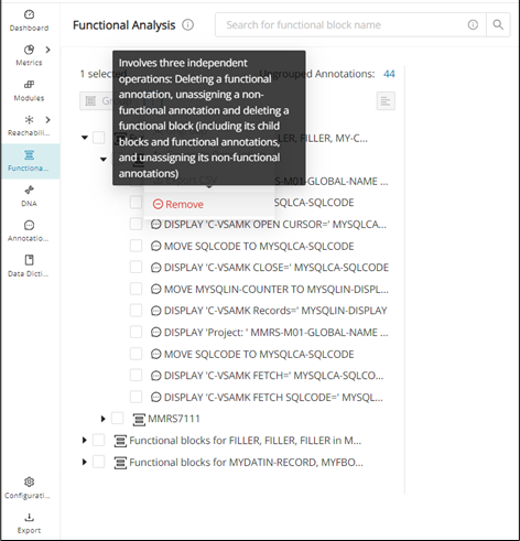
Sort
Sort the Functional Blocks in the "Functional Analysis" page by default order, name, last modified, only annotations, or by source order.
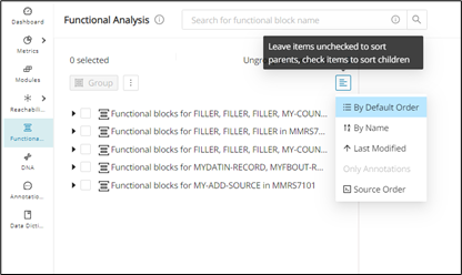
You can sort the children of a functional block in graph SQL queries. Functional blocks can be sorted by annotation offset, module name, and the presence of a functional group type. Additionally, it can sort individual blocks within the functional analysis tree.
The tree view will have an option to sort the children of a particular functional block. To do that, one needs to select the functional block and click the sort icon.
Bulk sorting is not allowed. Sorting will not be done recursively. Only the immediate children will be sorted. The children of any sub-block will not be sorted.
When the top-level sorting is done, it selects the current sorted option in blue.
The tooltip for the sorting button adapts to its state.
Enabled: "Leave items unchecked to sort parents, check items to sort children".
Disabled: "Sorting not applicable to the current selection."
The sorting within a selected functional block could be done either:
-
Default (Also covers re-ordering via manual drag and drop)
-
Alphabetically (ascending/descending)
-
Last Modified
-
Source Order
Sorting by Alphabetically, Last Modified, or Source code should not be persistent.
Details view
The Details View, which is the default view of the Functional Analysis page after creating at least one functional block, summarizes the selected functional block or annotation's description, related taxonomies, modules, data dictionaries, and annotations. You can switch between Process Flow, Control Flow, and Details View from the tabs located at the top right of the Functional Analysis page.

Details View for Functional Block
Editing Functional Blocks
Click the edit icon at the top of the "Details View" and edit the name and description of the selected functional block. The Functional Block name will update, and the description will update accordingly under the "Description" dropdown after saving changes in the Edit Functional Block modal.

The content in the details view of the functional block is segregated into different tabs.
The "Taxonomies & Modules" dropdown details the assigned taxonomies and modules in the functional block. Click See in Modules Table to open a new tab that shows the modules in the functional block within the "Modules" page.
The "Data Dictionaries" dropdown gives a preview of the data dictionary table in the "Details View". Click See in DataDictionary Table to open a new tab to see the Data Dictionary table of the functional block in the "Data Dictionary" page.
Finally, under the "Annotations" dropdown menu, you can open a saved search with the list of ungrouped annotations in a new tab when you click "unassigned annotations from used modules". You can also directly edit the annotations from the "Details View" by clicking on the edit icon.
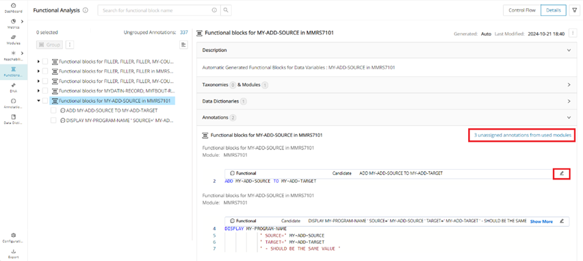
Details View for Annotations
The details view for annotations in the Functional Analysis page also contains "Additional Details", which contain both default and custom properties (if applicable). Please note, custom properties will only show if the selected annotation contains a value for the property. To learn more about custom properties for annotations, please take a look at Annotations Configuration.
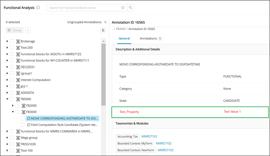
Process flow
The Process Flow view in the Functional Analysis page graphically shows a flow sequence of any selected functional block based on the executable process flow of the modules containing the functional Blocks. To access a functional block's process flow, select the desired functional block and then click the Process Flow tab at the top right.

Configuration
Empty functional blocks will have their Process Flow tab disabled.
Recalculate Process Flow
Grouped functional blocks within the selected functional block will show as expandable nodes with their own process flow sequences. Grouping changes in the tree view need to have the process flow restored to its default state by clicking Recalculate .
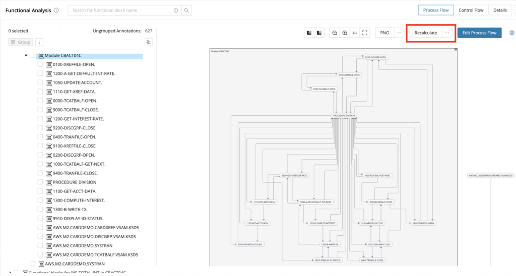
Recalculate gives the option to retain all manually created links in the graph in the following window.
To recalculate the selected functional block as well as its children, click Recalculate All .
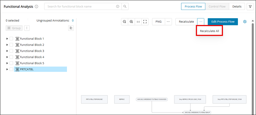
The following alert window will show after clicking Recalculate All . Click Recalculate after verifying.
Edit Process Flow
The selected functional block's process flow will display as a flow sequence. The process flow is view-only by default. To edit the process flow, click Edit Process Flow to open the edit window.
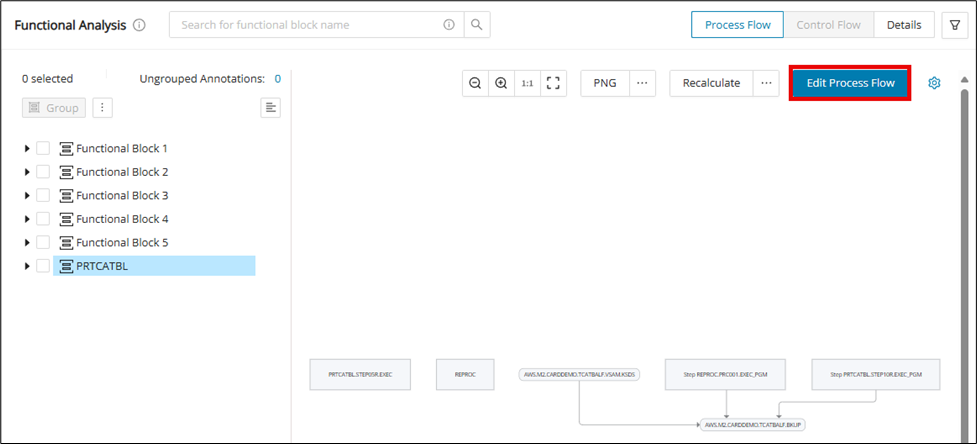
While editing the graph, it is also possible to change the shapes of the nodes to visually signal certain core operations happening along the process flow, including decisions and database Input/Output. Simply click on a node and hover over the edit node shape icon and pick the desired shape for the node.
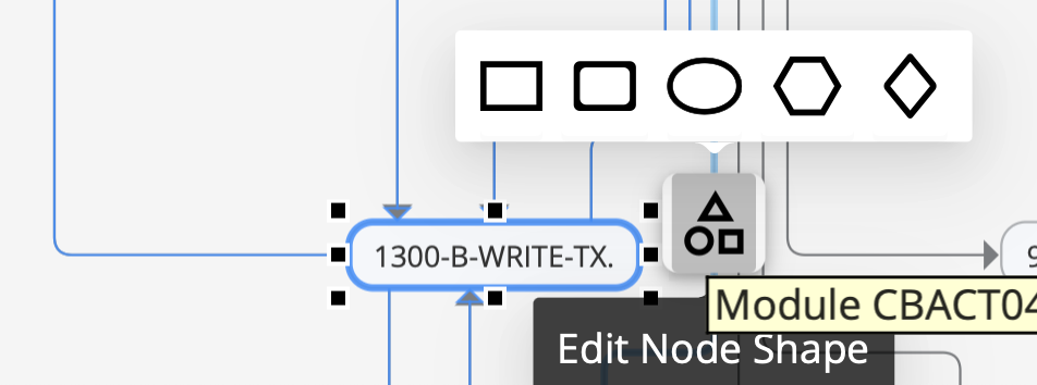
Click Save after making the necessary process flow changes.
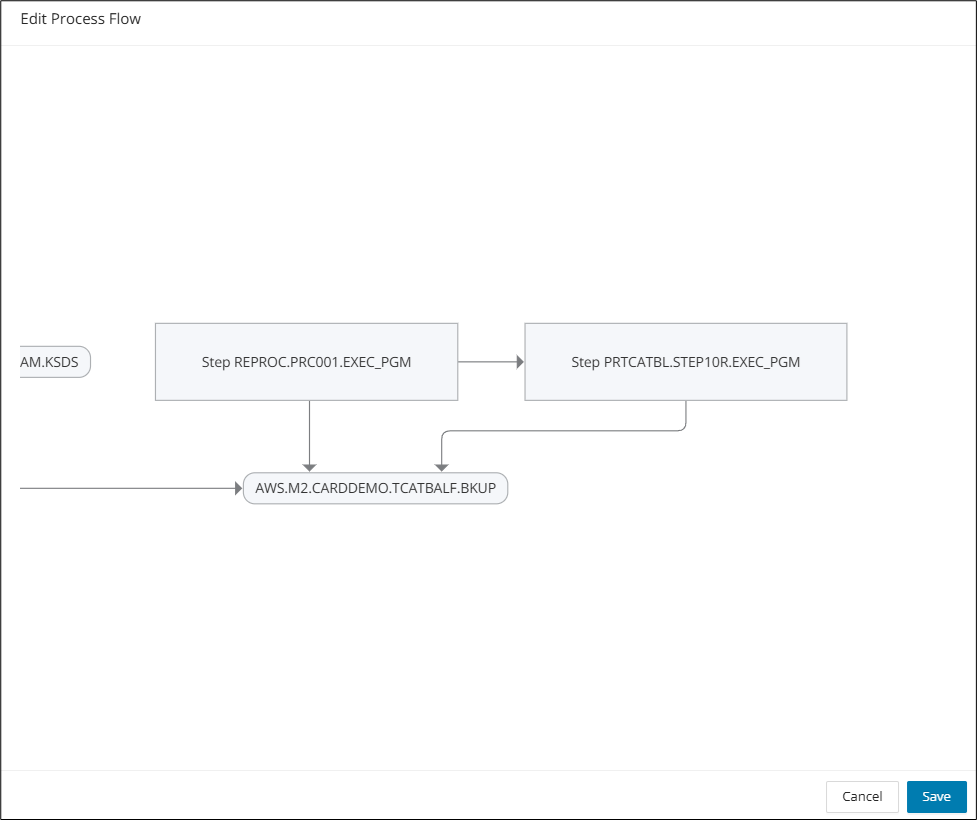
Show Annotations in Process Flow
To show/hide the annotations within the Process Flow, click the settings icon in the upper right corner to reveal the dropdown for "Show Annotations". When "Show Annotations" is enabled, all expanded functional block nodes display their contained annotation nodes within. Annotations are connected based on their configuration in the tree view.
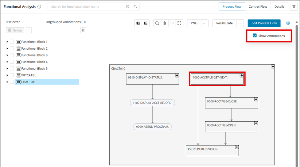
Expanded nodes containing annotations are shown below:
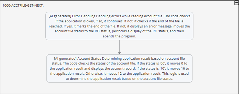
Control Flow
When the CFG node is clicked, the code viewer section, along with the relevant portion of the Code Viewer code, will be highlighted.
The side panel Code Viewer will have the double arrow buttons to expand and collapse the Code Viewer.
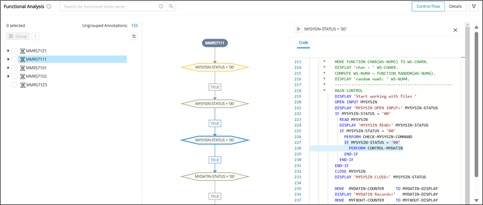
Configuration
Empty functional blocks will have their Control Flow tab disabled.
Search Control Flow Graph for structural and manual Functional Block
| Use Case | Control Flow Graph Visibility |
|---|---|
| Functional blocks created from annotation manual assignment that have all annotations part of the same module. | Visible |
| Functional blocks generated via Reachability Analysis. | Visible |
| Functional blocks generated via the Module Structure approach. | Visible |
| Functional blocks generated via the Semantic Functional Block approach. | Visible |
| Functional blocks generated via the Field Level Mining approach (CodeViewer or Data Dictionary). | Visible |
| Functional blocks generated via the Field Level Mining approach (CodeViewer or Data Dictionary), and if a new annotation from the same module gets added to the block | Visible |
| Functional blocks generated via the Field Level Mining approach (CodeViewer or Data Dictionary), and if a new annotation from a different module gets added to the block | Visible |
| Functional blocks generated via the Field Level Mining approach (CodeViewer or Data Dictionary), and if a new annotation from a different module gets added to the block | Visible |
The disabled Control Flow will have a tool tip mentioning that the button has been disabled, as the graph cannot be generated.
Control Flow for manual Functional Block
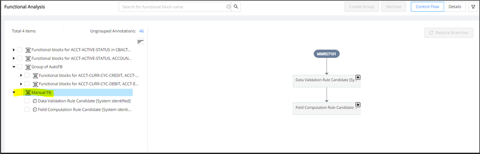
Control Flow for structural Functional Block
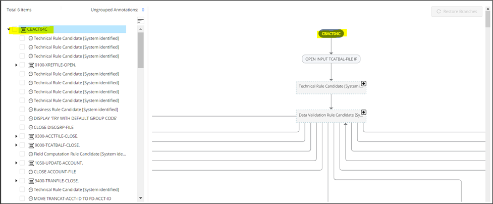
The collapsible on the graph will be shown for the Functional Group's direct children of the selected group. Inside this collapsible, you will see all children with no more collapsibles inside (you can see the collapsible only at one level).
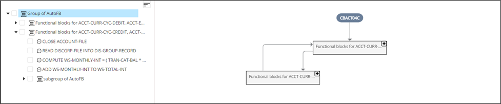
Filter
With this function, users can apply any filter or combination of filters to get the functional block(s) associated with the criteria.
The Functional Analysis window displays filters for:
-
Taxonomy
-
Reachability Block
-
Module Name
-
Data Dictionary Entry
Multiple options can be selected from the four filter drop-down lists.
To apply the filter function:
Step 1:
Click the filter icon.
The Functional Analysis window opens, displaying all filter options.
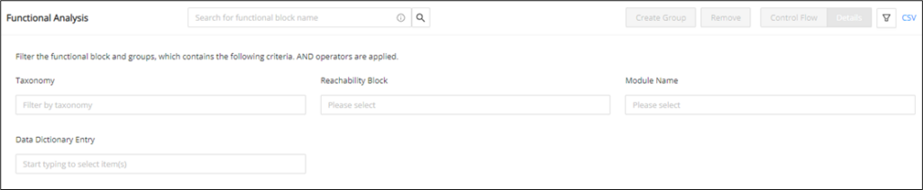
Step 2:
Select the appropriate option(s) from the Taxonomy drop-down list.
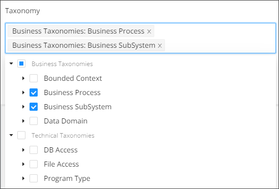
Step 3:
Enter the name of the reachability block(s) and select the desired option from the drop-down list of the Reachability Block.
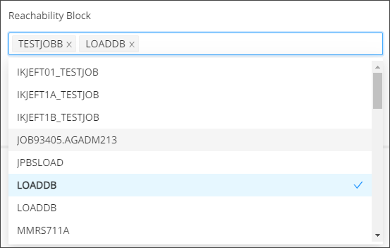
Step 4:
Enter the name of the module and select it from the drop-down list of the Module Name filter.
Step 5:
Enter the name of the data dictionary and select the desired option from the drop-down list of Data Dictionary Entry. The functional blocks with the mentioned data dictionary will be filtered.
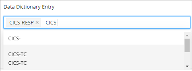
Step 6:
To clear the selection, click Reset

Navigation from Reachability Blocks
This functionality allows the user to view all of the functional blocks associated with the respective reachability block.
To view the referenced functional blocks:
Step 1:
Click the green badge icon shown below on the reachability block.
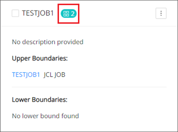
Step 2:
The user will be redirected to the Functional Analysis page that displays the functional blocks associated with the reachability block.
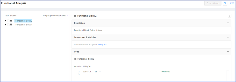
Step 3:
The Reachability Block filter will be populated with the block name.

Search Functional Blocks inside tree view on Functional Analysis page
Functional blocks within the tree structure can be searched on the Functional Analysis page. The user can search functional blocks by full name and with wildcards. Hover over the tooltip icon for the Wildcard Syntax.
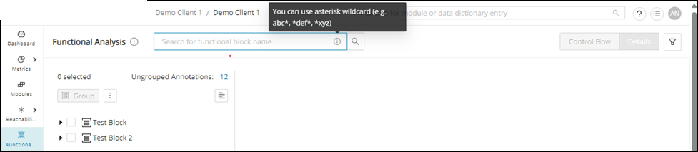
Blocks available inside a functional group can also be searched with full name and wildcards.
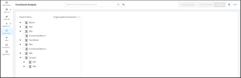
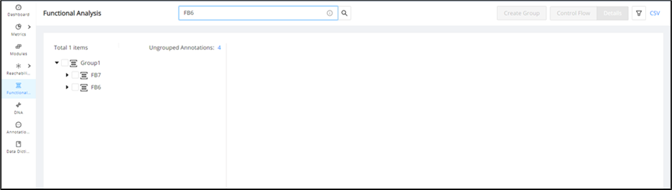
Custom properties for Functional Blocks
Further customize the output of your Functional Analysis by using Custom Properties. Similar to the use of custom properties across Mining, you can create custom String Input, String Repeater, URL, and Select Tag fields and edit them for each Functional Block to provide additional context, for example, (industry or client-specific meaning surrounding the source code).
Step 1:
Configure your custom property(s) scoped to Functional Blocks from the Configuration page.
Step 2:
Populate the custom property when creating a new Functional Block manually or when editing an existing Functional Block.
Adding Custom Properties during Functional Block creation:
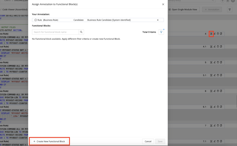
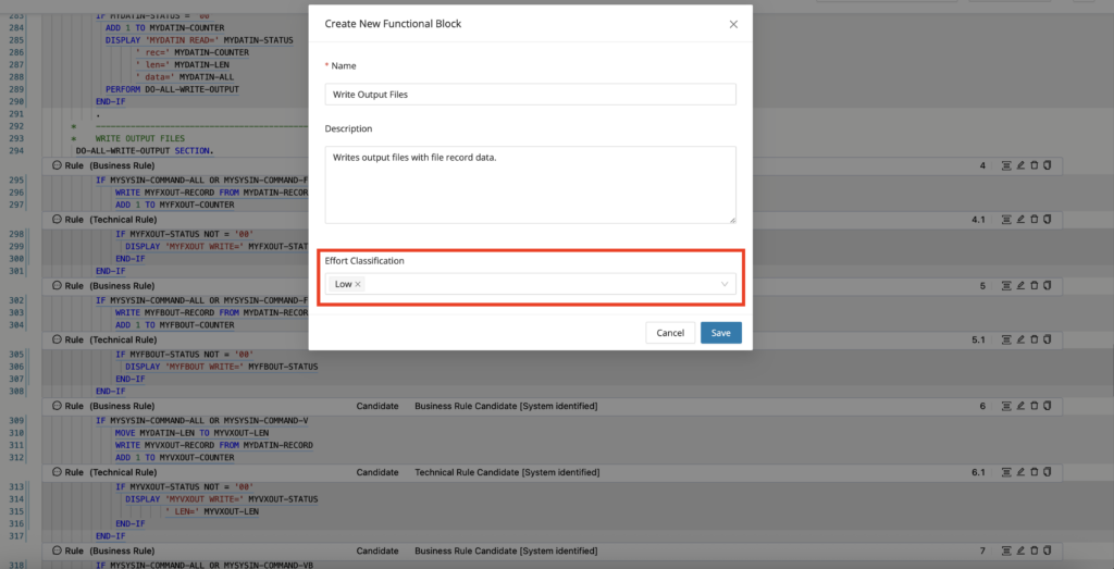
Adding or editing Custom Properties during Functional Block editing:

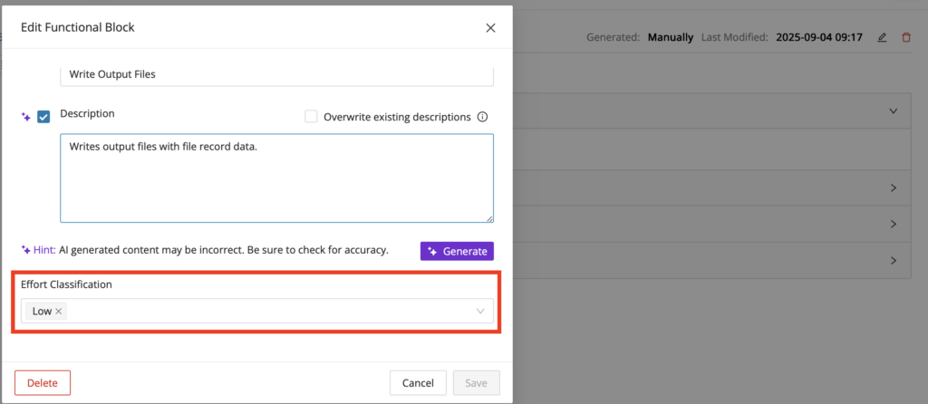
Data Lineage
Data Lineage provides insights into the data flow of an application to address key modernization challenges (data migration, impact, and compliance). This feature traces the data flow of your selected data entity (for example, variable, table column, etc.), and allows you to easily answer questions such as "If I remove a SQL Table column, which programs throughout my application would be affected?" or "How is the data consumed throughout my application from a resource file?".
Info
Only Cobol and SQL are supported for Data Lineage.
Data Lineage visualization
Data Lineage visualization shows how selected fields and statements connect across modules and interfaces. The graph views help you move from a single field reference to a broader understanding of upstream and downstream impact. Use the subsections below to open the visualization from the two main entry points.
Graph visualization from CodeViewer
Please follow the following steps to view the Data Lineage graph for a variable from the Code Viewer:
-
Place the cursor on a variable (either where it is declared or referenced in code).
-
Right-click and select the Show Data Lineage option from the context menu.
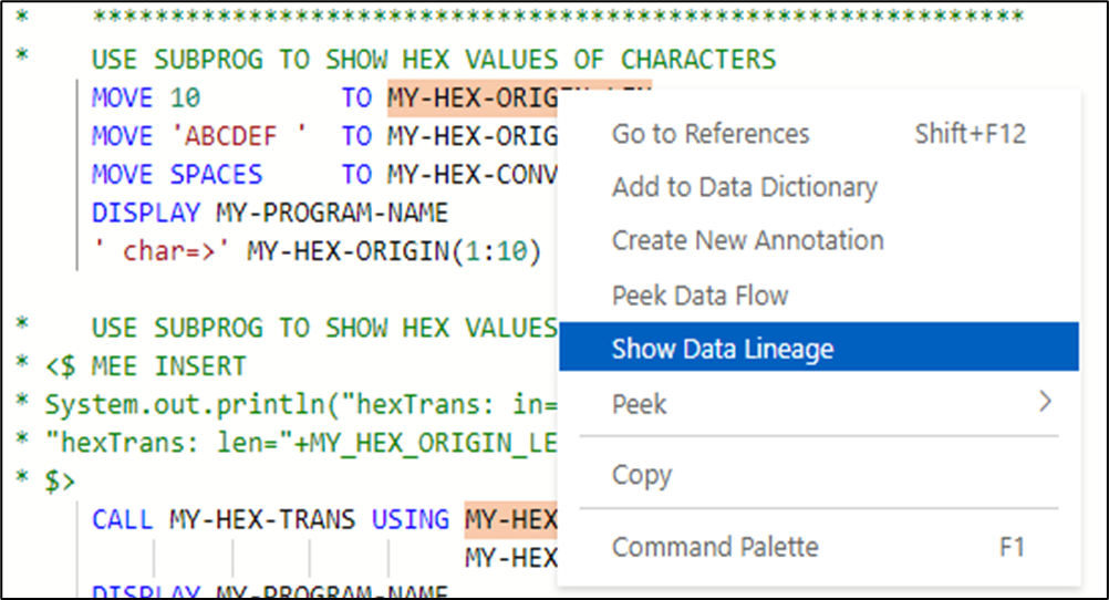
-
User is directed to a new tab with a scrollable graph (horizontal/vertical) for its data lineage.
-
The graph can be zoomed in and out using the two magnifier buttons displayed at the top right corner of the page.
-
Nodes of one module are grouped.
-
The graph will display only the immediate upstream (including all the data flow that enters the selected field via related fields) and downstream data flow from the selected field.
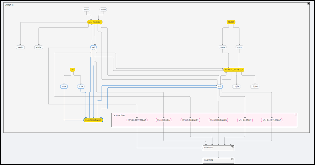
- Clicking the icon of a module node will display the internal intra-module data flow of the module.
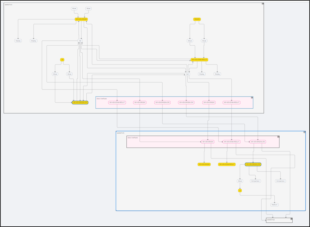
-
Statements, Fields, and Data Interfaces in the graph are differentiated by color coding:
-
Statements: white
-
Fields: yellow
-
Data Interfaces: pink
-
Info
Data interfaces are the gateways for data flow between modules. They show exactly how each data element comes into a module or leaves a module, going elsewhere across the codebase.
Graph visualization from the Data Dictionary
To trigger Data Lineage on any supported Data Dictionary entry, click on the menu icon of the Data Dictionary entry and select the "Open Data Lineage" option.
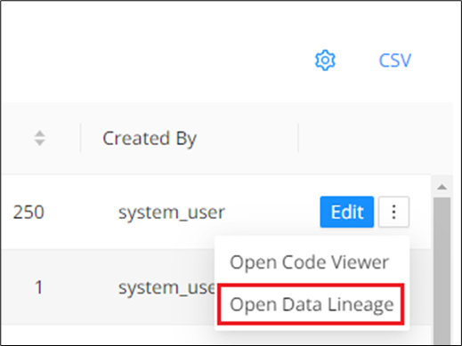
The Data Lineage graph will be displayed in a new tab.
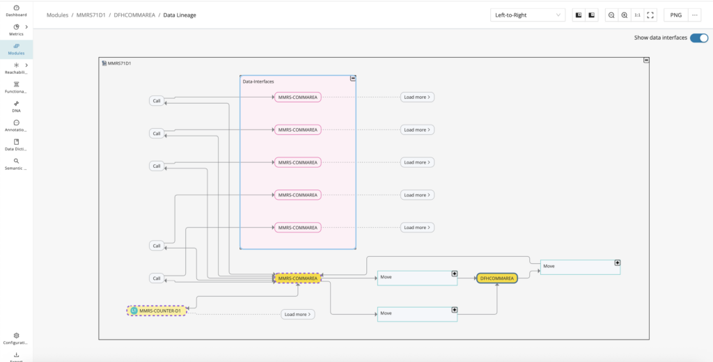
Iterative data flow loading
Iteratively expand the graph to trace data flow for your selected fields across the codebase. By default, the graph will load the immediate intra-module data flow for the initially selected field node. From here, you can click the load more button in various directions to trace the data flow within your starting point module and across modules, going as far across the codebase as needed.
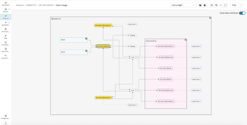
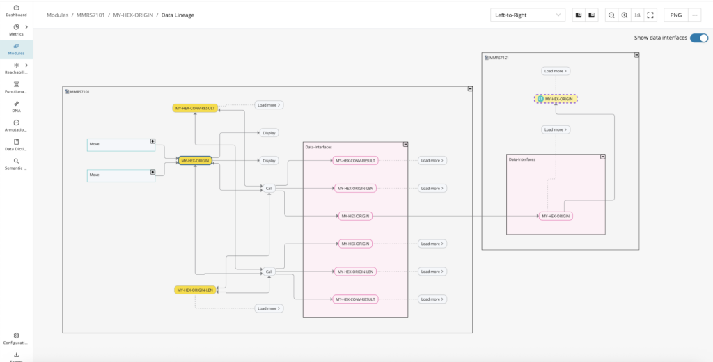
Module overview panel
The side panel of the selected modules displays when any grouped module node is clicked. The side panel has details such as the module name, path, base data (which consists of technology/type), metrics (which consists of total source lines of code/comment lines of code/complexity level), description, custom properties, taxonomies, and annotations.
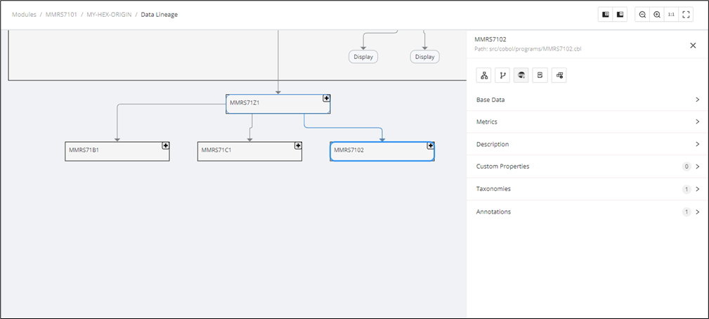
By default, clicking on a module node will show the Module Details tab on the Modules Overview panel. In the case that this Module node is a SQL table node and the associated DB schema has been uploaded, or a SQL script outlining the schema has been discovered, an additional SQL Details tab will be shown.
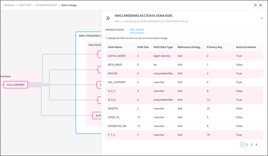
Source code panel
To display the underlying source code that corresponds to a particular field or statement node within the data flow path on the graph, simply click on the field or statement node. From there, click the side panel icon and the source code panel will appear positioned to the line of code where the field is declared or the statement transformation occurs on the opened side panel.
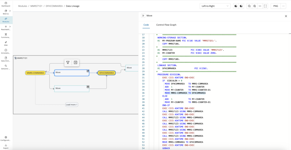
By default, when you click the side panel icon, you see the code tab on the panel that opens. Toward the top of the panel, you can also select the Control Flow Graph tab to see the executable control flow of a statement node, including any conditions or preconditions that must be evaluated before that statement is executed, providing you with greater context without having to manually analyze the source code.
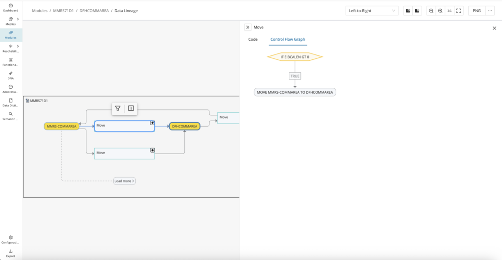
Filtering the graph
As the Data Lineage graph can grow to become quite large after expanding the data flow, there are filtering options available to make it easier to cut through the noise and focus on just the data flow paths or clusters of nodes that are of interest. These filters help isolate the part of the lineage that matters for the question you are investigating. Use them when the full graph becomes too dense to review efficiently.
Show path of neighboring nodes
From the Data Lineage graph, it is possible to get a view of just the nearest neighbor nodes or a node you have selected to see this cluster in an isolated view. Simply click on the field or statement node of interest, and from there, hover over the icon and select "Show path of neighboring nodes".
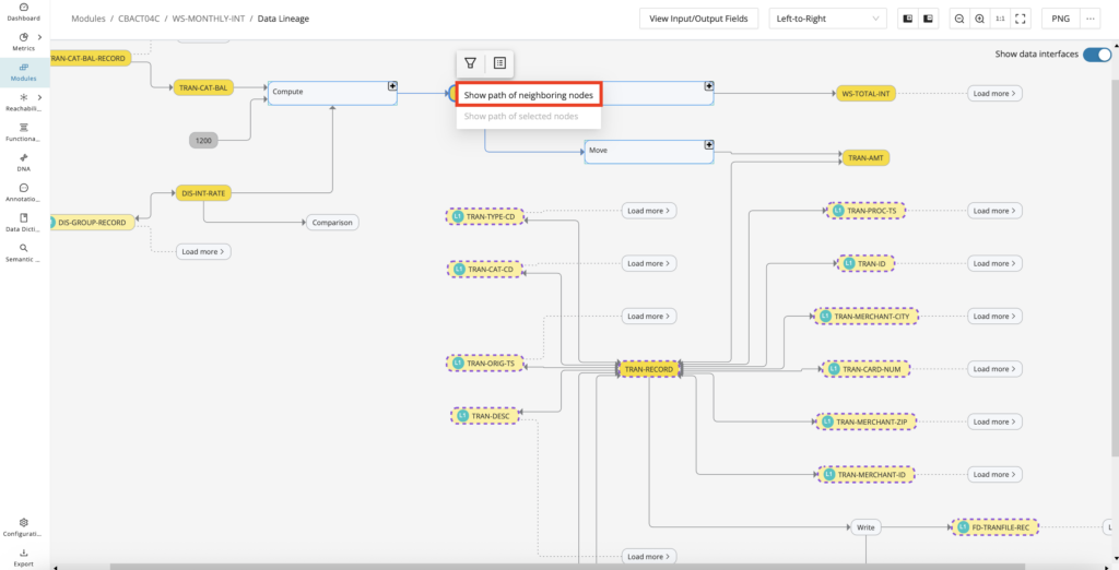
On the pop-up modal, which shows the nearest neighbor nodes of your selected node, the graph view defaults to a depth of 1, but you can configure it on the top right up to a depth of 10. Additionally, you can zoom in and out and export an image of the graph view similar to the main Data Lineage graph.
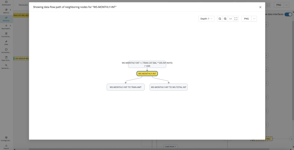
Show path of selected nodes
From the Data Lineage graph, when there is a need to analyze the end-to-end data flow path between two nodes, it is possible to filter and extract a view of this single path. Simply click on the "starting point" field or statement node of interest, and while pressing the Control key (Windows)/Command key (Mac), click the "ending point" field or statement node of interest. From there, both selected nodes should be highlighted in blue, and you can hover over the icon and then select "Show path of selected nodes" to see the end-to-end path between your starting and ending selected nodes.
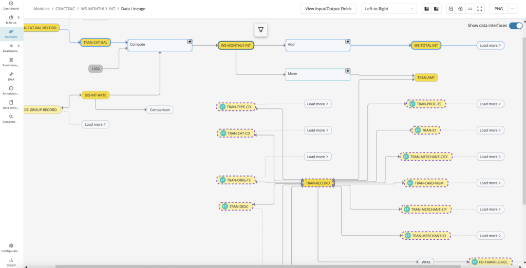
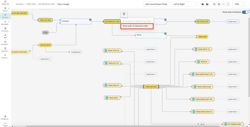
On the pop-up modal, which shows the data flow path between your starting and ending selected nodes, you can zoom in and out and export an image of the graph view similar to the main Data Lineage graph.
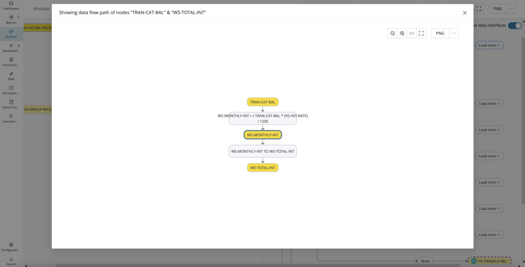
Input/output fields
To display the input and output fields associated with read and write statements, click the View Input/Output Fields. When clicked, a new tab displays the data dictionaries related to those fields. To change the layout of the Data Lineage to either the default left-to-right layout or a hierarchical layout, click the dropdown menu shown in the middle of the Data Lineage window.

If no Data Dictionary entries are present from "View Input/Output Fields", an error warning message will be displayed as below.

Exporting graph image
The image export button on the top right has been added to the Data Lineage for export options. PNG(default), GraphML, PDF, and SVG are image formats supported. The Export file name will use the following naming convention: "DataLineage_For_[FieldNameHere]".
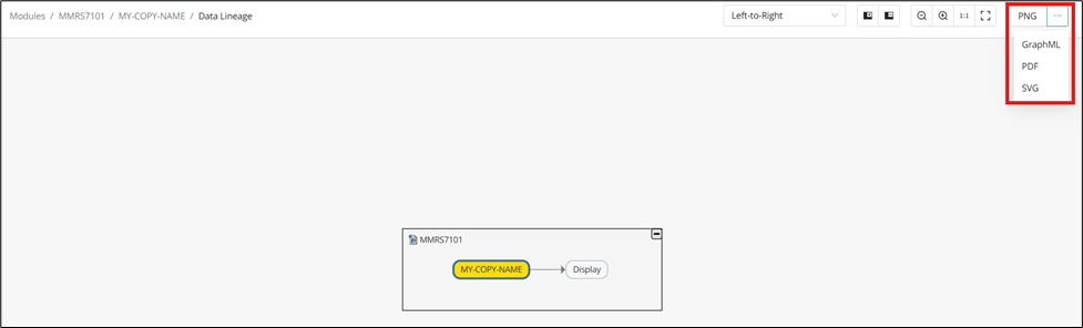
Data interface toggling
To show or hide data interfaces, toggle "Show data interfaces" on the top right. This toggle helps you switch between a fuller integration view and a cleaner field-to-field view of the graph. Use it when you need to confirm whether interface nodes are adding necessary context or just visual noise.
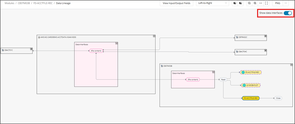
DNA
Code Discovery & Mining empowers teams to accelerate modernization by identifying code patterns known from the source modules. Through DNA analysis, the platform examines each statement as a building block, grouping modules with similar structures into clusters. Once a pattern is found in one module, similar modules within the cluster can be quickly identified and analyzed. Users can interact with clusters, view associated modules, and leverage snapshots to track changes and version history.
The DNA page visualizes the data gathered by the Discover DNA feature (see Discover DNA) or by clicking Analyze directly on the DNA page.
Info
This feature is available for C, COBOL, JCL, Natural, and PL/I.
The DNA analysis looks at the statements of each module and searches for patterns. Each statement is considered a building block of the code. Identified clusters represent modules with a similar DNA.
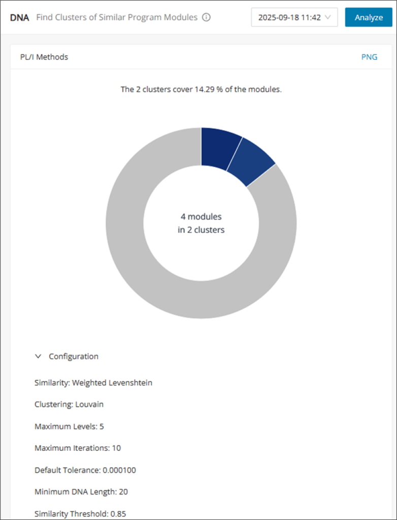
After performing DNA Analysis, the DNA page will populate with a chart of the results, as well as a version history drop-down and the Analyze button in the top right corner. When a change is found from subsequent DNA Analyses, a new version will be recorded in the version history.
Cluster table view
Clicking on different parts of the chart returns different table views, which can be customized and used for CSV or Confluence export. These table views let you pivot from the cluster visualization into the underlying module lists. Use them when you need exportable detail for either the full dataset or a single cluster.
-
Clicking the blank area of a chart opens an overlay table listing all modules.
-
Clicking one of the clusters opens an overlay table with all of the modules of the chosen cluster.
-
Clicking the unassigned, gray cluster opens an overlay table of the modules that were not assigned to a cluster.
Click on the settings icon to customize the table view and then click on CSV/Confluence to export.
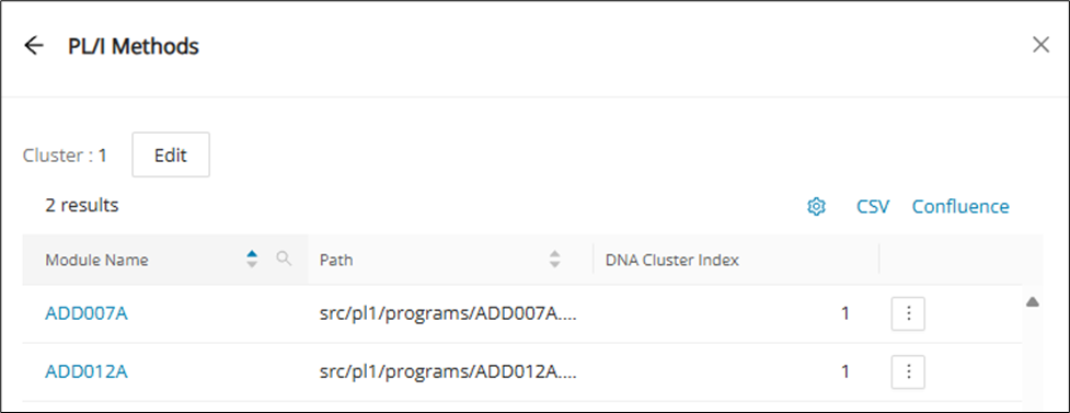
In the cluster's table view, each listed module in the table has a menu to open its Code Viewer, Control Flow, or Dependency Graph page in a new tab directly:
Edit cluster
Cluster names are automatically assigned to their DNA Cluster Index (starting from 1), but can be renamed and given a description to your liking. Click Edit at the top of the cluster's table view.
Info
Modules without a cluster do not have a DNA Cluster Index.
Input the name and description (optional) and then Save .

Edit DNA configuration
DNA configuration is performed from the Eclipse project files. For more information on DNA configuration, find more details under Discovery with Customized Settings.
Annotations
Annotations encapsulate metadata about a snippet of code to provide insights into its purpose. Together, they form the foundation for documenting the functionality of a system, especially when combined into Functional Blocks. The Annotations page allows you to view and work with annotations. It displays a list of all available annotations that can be narrowed down according to your search and filter criteria for each column.
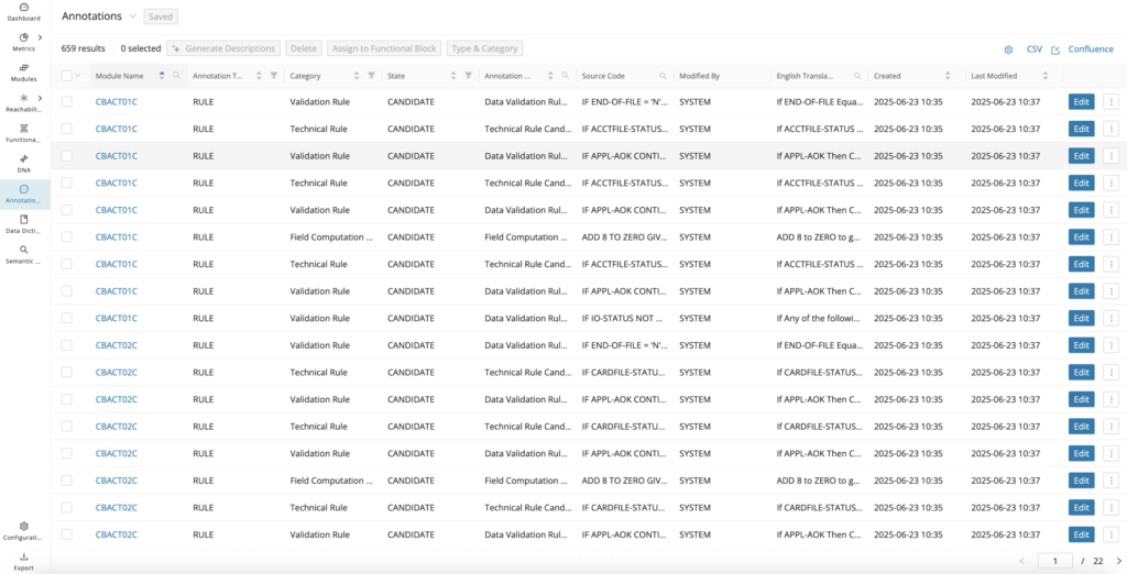
The annotation table provides extensive insight into the project's annotation details. The visible columns can be adjusted using the settings icon in the top right corner.
Click the up and down arrows in the column headers to sort the result list. To refine the search, select specific values for the respective columns via the filter or search icons.
Once the desired annotations are displayed, export the list by clicking CSV in the top right corner.
You can edit the description and state of annotations displayed in the result. Click Edit of the corresponding annotation list entry to open an Edit Annotation Details dialog. Subsequently, enter the description, select the appropriate state from the drop-down list, and click Save .
Open the shortcut menu next to Edit to directly open the Code Viewer for the corresponding module at the position of the selected annotation.
Annotation identification reasoning
When auto-generating annotations, the system justifies why Rule Type annotations were categorized a certain way, for example, (business rule vs technical rule). On the Annotations page, select Identification Reason from the setting options to display a new column with the Identification reasoning types and tags.
Info
Requires executing Identify Candidates to auto-generate the annotations with the Identification Reason data point populated. This feature is currently only supported for COBOL.
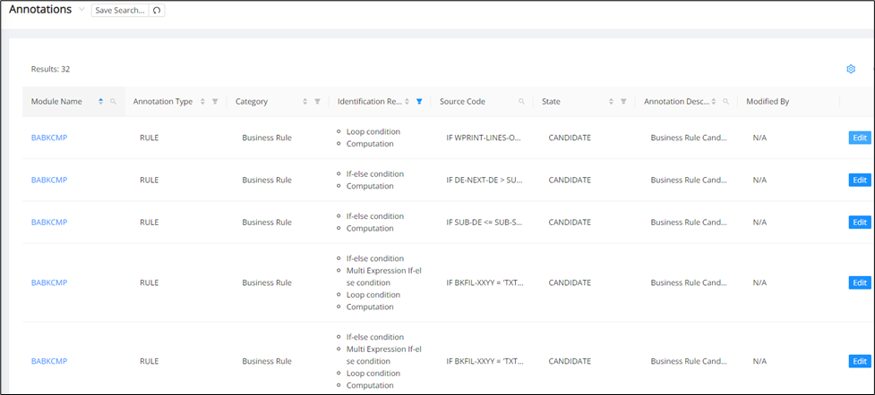
The identification reasoning Types are Conditions, Actions, and Nesting, and the relevant tags are mentioned below:
| Conditions | Actions | Nesting |
|---|---|---|
| If-else condition | Computation | Nested Condition |
| Multi-expression | Input from an external data source | |
| Loop condition | Output to external data source | |
| Cobol Evaluate condition | ||
| Natural Loop File Access condition | ||
| Select condition | ||
| Other condition |
Info
For Nesting, multiple identification reason types can be used per Candidate. For example, a nested If-else will have both a Nested condition and an If-else condition.
Annotation types and categories
Annotation Types are used to place annotated code into main categories, while Annotation Categories are used to further classify annotated code beyond their Type as needed. These help with sorting and filtering the annotations and quickly identifying their relevance among different areas of the system. Type Rule and Database Annotations are generated via Identity Candidates. Type Dead Code via Identify Dead Code, and Type Functional via Identify Functional Block or Identify Candidates.
The following table provides an overview of each of the Annotation Types and Categories:
| Types | Categories | Description |
|---|---|---|
| Database | Close | Signals a database connection closing annotated statement. |
| Declare | Signals a declare cursor annotated statement. | |
| Read | Signals a read, for example, (File/Database) annotated statement. | |
| Write | Signals a write, for example, (File/Database) annotated statement. | |
| Dead Code | None | Signals that the annotated statement(s) will never be executed during runtime. |
| Exclude | None | Signals that the annotated statement(s) are not in scope for the Mining project or can be ignored (Manual assignment). |
| Functional | None | Signals that the annotated statement(s) were generated via Functional Analysis and do not use the heuristics of Identify Candidates. |
| Action | Signals that the annotated statement(s) are executable statements inside of a conditional block and are generated via Identify Candidates. | |
| Condition | Signals that the annotated statement(s) are conditional statements that encapsulate executable statements and are generated via Identify Candidates. | |
| Rule | Business Rules | Signals that the annotated statement(s) represent a business obligation regarding some conduct, action, practice, procedure, or compliance within a key business activity or process. |
| Error Processing Rule | Signals that the annotated statement(s) form decision statements that take into account whether the application is in a state of error before proceeding to take some error handling action(s). Consists of both decision and action statements. | |
| Field Computation Rule | Signals that the annotated stand-alone action statement(s) reference input/output variables to execute some computation and produce an output. | |
| Process Rule | Signals that the annotated statement(s) are part of an executable process flow (Manual assignment). | |
| Technical Rule | Signals that the annotated statement(s) form decision statements that take into account the technical state of an application/system, which is based on the programming language/syntax for an application, before proceeding to take some action(s). Consists of both decision and action statements | |
| Validation Rule | Signals that the annotated statement(s) form decision statements that do a comparison check against the internals of a non-business variable(s) to validate the data before proceeding to take some action(s). Consists of both decision and action statements. |
English Translation data point
The English Translation feature allows the user to understand any annotated COBOL code in plain English by adding the default English Translation column to the Annotations table. It helps reviewers interpret annotation logic without reading every original statement in COBOL syntax. Use it to compare technical expressions with a more business-readable rendering before validating the annotation.
Info
This feature is available for COBOL only.
Info
From the annotation table or editor, you can see referenced business or non-business variables linked from the Data Dictionary. Open the linked Data Dictionary Entry in the Data Dictionary Editor and update the Translated Field Name field to give a more meaningful name to the variable, which will be used in the English Translation of the associated annotation, making the English Translation more meaningful as well.

The English Translation feature only supports annotations with type RULE and is visible from the Annotation tables and also in the Annotation Editor.
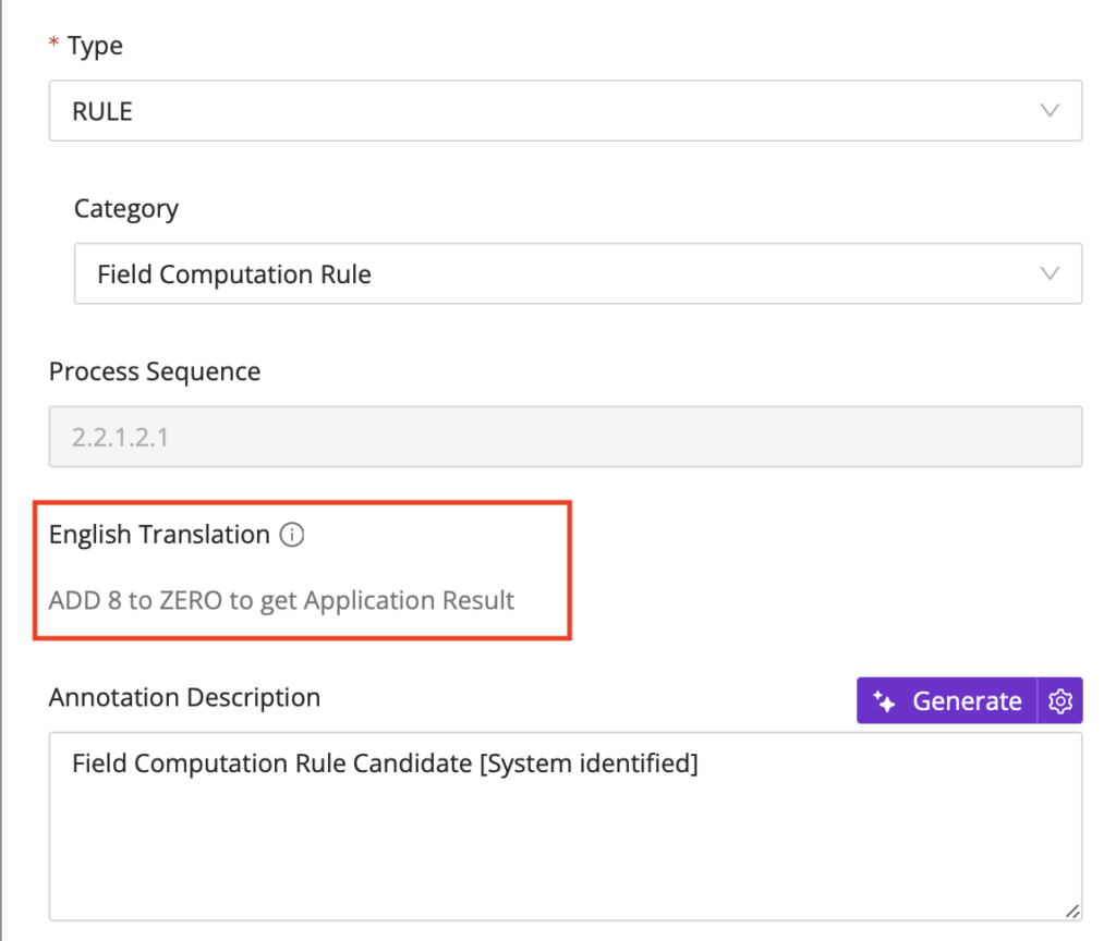
The English Translation feature supports all of the RULE candidates, including:
-
Business Rules
-
Technical Rules
-
Field Computation Rules
-
Validation Rules
-
Error Processing Rules
For comparison expressions, the translation appears as follows:
-
> Greater than
-
>= Greater than or equal to
-
\= Equal to
-
< Less than
-
<= Less than or equal to
For arithmetic expressions, the translation appears like in the following examples:
-
ADDITION: ADD WS_A, WS_B to WS_C == Add WS_A and WS_B to WS_C to get WS_C
-
SUBTRACTION: SUBTRACT WS_A, WS_B from WS_C == Subtract WS_A and WS_B from WS_C to get WS_C
-
MULTIPLICATION: MULTIPLY WS_A, WS_B by WS_C == Multiply WS_A and WS_B by WS_C to get WS_C
-
DIVISION: DIVIDE WS_A, WS_B by WS_C == Divide WS_A and WS_B by WS_C to get WS_C
For expressions with logical operators, the translation appears as follows:
-
&&/&/AND = AND
-
|| / | /OR = OR
-
!/NOT = NOT
Conditional and Action statements should be translated as shown below:
- If/Evaluate/Case type conditional statements with a single expression, the translation appears as follows:
if
-condition here
Then
-actions here
- If/Evaluate/Case type conditional statements with multiple expressions translates as follows:
if any of the following conditions are true:
-expression1 here
-expression2 here
....
Then
-any actions here
- For/Do/While looping conditional statements with a single expression, the translation appears as follows:
while
-expression here
Do
-any actions here
- For/Do/While looping conditional statements with multiple expressions translates as follows:
while any of the following conditions are true:
-expression1 here
-expression2 here
....
Do
-any actions here
Dynamic field names are those that are not field names/data dictionary entries in the data dictionary table and will be italicized in the translation.
In the English Translation output, if there are linked Data Dictionary entries whose Translated File Name attribute is populated (From the Data Dictionary Editor) to provide a more meaningful name, it will be used in the place of the defined field name.
Business Variables referenced
To display the column “Business Variables Referenced”, click the settings icon in the top right corner and select Base Data > Business Variables Referenced. This view highlights which business-related data elements are tied to each annotation. Use it when you need to trace business context from a rule candidate back to the supporting Data Dictionary entries.
The column contains field names and links to each business-related Data Dictionary entry after the identification of candidates from the Modules Reporting page.
Field names and links are displayed only for Annotation candidates of Type "RULE" and Category "Business Rule".
The Data Dictionary editor contains a tab "In Business Rules" with a list of all associated Candidate Business Rules for the corresponding field name. This link is bi-directional, so that the edit icon of each entry in the tab opens the associated Annotation editor for each annotation.
Annotation copying and pasting
In case you would like to manually duplicate annotations across similar code/programs, you can do this using the copy and paste functions for annotations. Copying saves the contents of an annotation to your clipboard so that you can quickly select another snippet of code, create a new annotation, and paste in those saved contents.
Copy Annotation
You can copy an annotation from several places in the UI (for example, from Annotation Tables, the Annotation Editor, or the Code Viewer). Each option copies the annotation’s full details to your clipboard so you can paste them into another (existing or newly created) annotation to quickly duplicate the same configuration.
Click on the menu icon of the annotation you would like to copy to open a drop-down menu. Then, click Copy .
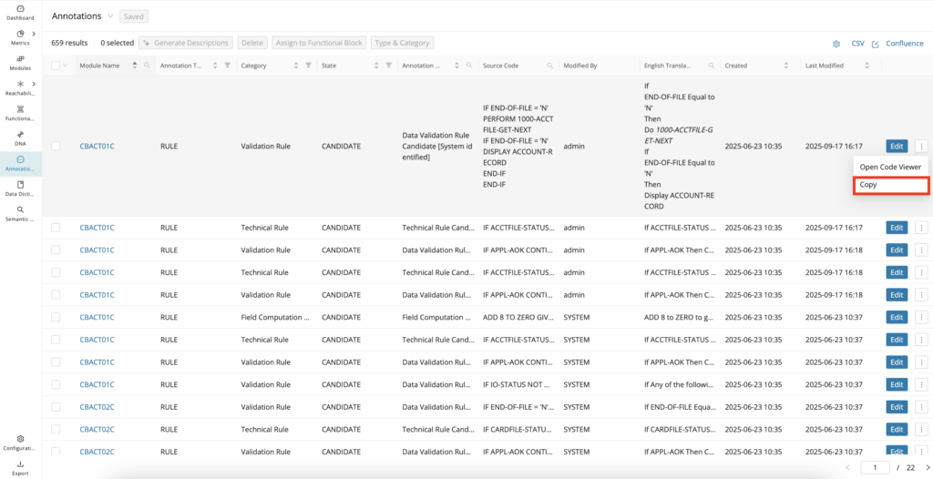
Open the annotation editor for the annotation you would like to copy and click Copy Details .
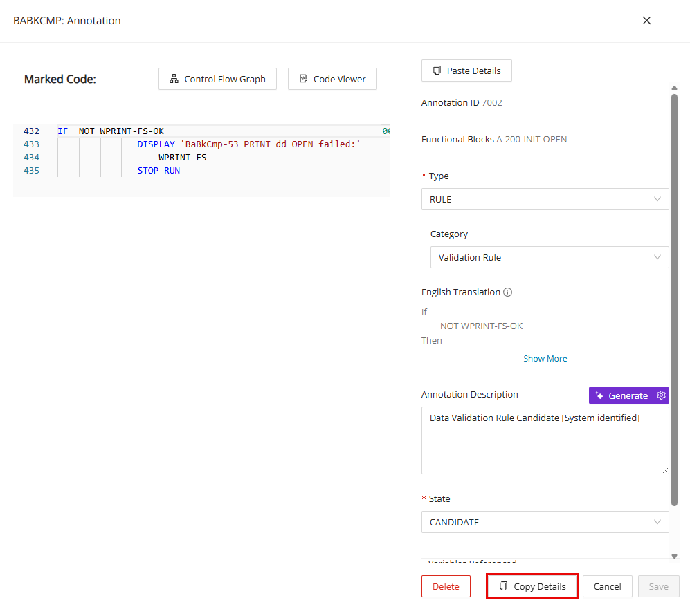
Open the Code Viewer and click on the edit icon of the annotation you want copied. Click Copy Details to copy the annotation. Using this copied annotation, you can Paste Details by either finding another annotation or creating a new annotation to paste the details. See Managing Annotations in Code Viewer for more context.
Paste Annotation
After you’ve copied an annotation, you can reuse it by pasting the saved details into another annotation from either the Annotation Editor or the Code Viewer. Open (or create) the target annotation, then click Paste Details to populate the fields with the copied content; review and adjust as needed, and click Save .
Annotation custom properties
Annotation custom properties let you extend the metadata captured for annotations beyond the built-in fields. They are useful when a project needs client- or domain-specific attributes to support filtering, review, or export. The subsections below describe how categories and mandatory behavior work.
Custom property category
This feature allows the user to select from a drop-down of custom properties categories, which displays the category of custom properties they'd like shown on the annotation editor, and on this basis, custom properties are displayed on the Annotation Editor. When one Custom Property Category is selected on the Annotation Editor, other Custom Property category fields are hidden, and by default, all custom properties scoped to annotations are shown.
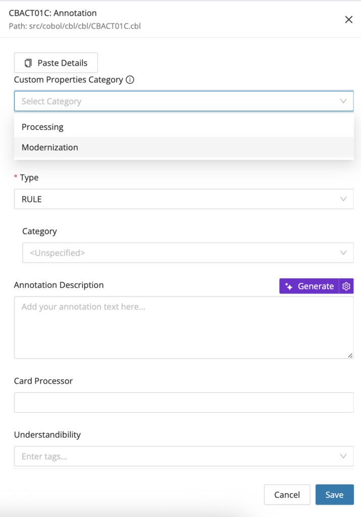
Mandatory custom property
The mandatory checkbox has been added in the custom property editor along with an info icon and a tooltip.
If made mandatory, the custom property is made required in the Annotation Editor. The Save button is enabled and disabled based on the validation of the mandatory field.
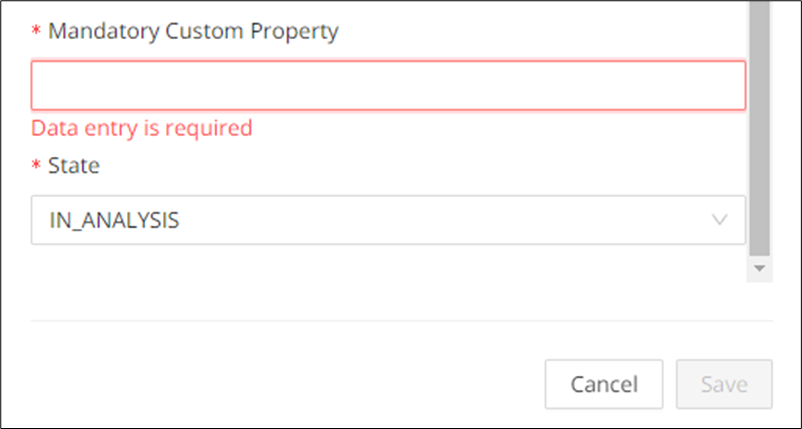
Bulk generation of Annotation description
Bulk generation of Annotation description lets you create GenAI-assisted descriptions for multiple annotations in one action. It is useful when you want to accelerate first-pass documentation across a filtered result set. Review the generated text afterward, especially when existing descriptions may be overwritten.
Configuration
The feature toggle generativeAiTranslations must be enabled in the WebUI feature console.
Step 1:
Select all the annotations for which bulk description generation is required and then click Generate Descriptions . The user can overwrite the existing annotation descriptions by selecting those annotations as well.
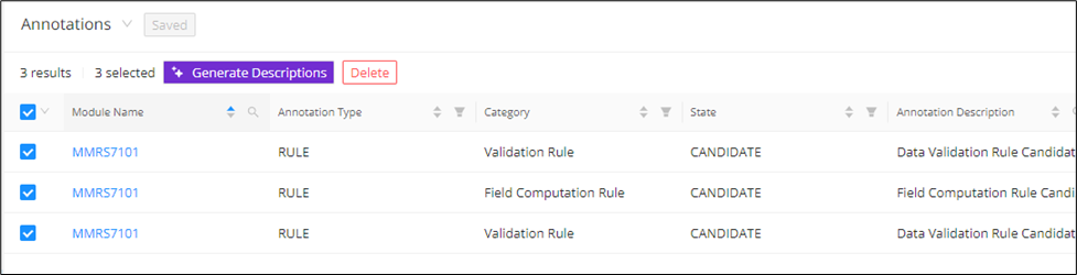
Step 2:
Click Generate Descriptions on the pop-up.
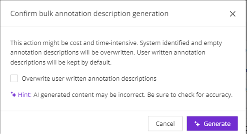
As a result, the annotation descriptions for all of the selected annotations are generated with "[AI generated]" before the description.

Edit Annotation type & category
Individually updating each annotation's type and category can be time-consuming and error-prone. To streamline this process, navigate to the Annotations page and select one or more annotations, and click Type & Category .
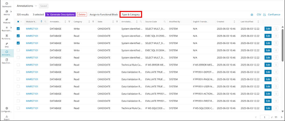
Select the Type and Category and click Save .
Advanced AI options
There are times when GenAI produces annotation descriptions that are too technical, contain inaccuracies, or require more context. The "Advanced AI Options" modal is where you can provide more context to the prompt and expect better generated results for the annotation description. Some context retrievers that are used by default to provide more meaningful descriptions are:
-
Lines of code before and after an annotation
-
Functional Block: the annotation is part of
-
SQL tables that are accessed in an annotation
-
The name of the module the annotation is part of
Find the "Advanced AI Options" modal from any annotation's edit page. Click the settings icon next to Generate .
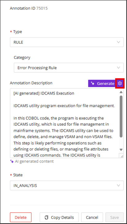
Add any additional industry, client, or codebase-specific context to help generate more meaningful annotation descriptions in the "Advanced AI Options" modal that displays, and then click Add Context .
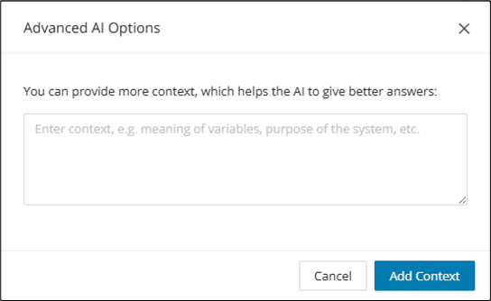
Data Dictionary
The Data Dictionary acts as a single domain data entity repository for storing metadata about the data for your codebase. This includes program and Copybook fields, BMS Map fields, SQL columns, and File Record Layout columns (extracted via COBOL field declarations). This Data Dictionary works hand in hand with annotations to provide greater context on the overall codebase, providing insights into the industry/client-specific data entities. All entries can be narrowed down according to your search and filter criteria for each metadata column to support quick data lookups.
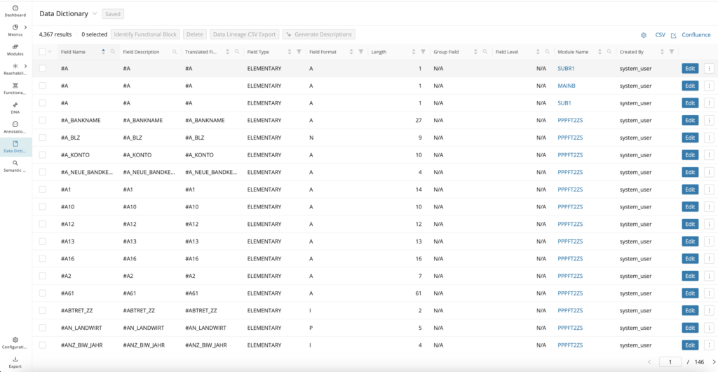
The data dictionary table can be customized via the settings icon in the top right corner.
Click the and arrows in the column headers to sort the result list. To refine the search, select specific values for the respective columns via the filter or search icons.
Once the desired data dictionary entries are displayed, export the list by clicking CSV in the top right corner.
Linking Data Dictionary entries
Data Dictionary entries can be linked together to form a larger data meaning. For example, you can link entry fields that are synonymous with each other or fields that share a file record layout to provide a layered context around these data entities. At the time of linking, it is possible to give them a meaningful group name that can be searched within the Data Dictionary tables.
Info
It is possible to have linked Data Dictionary entries be part of multiple groups of linked entries for maximum flexibility.
Creating a new group of linked entries
Step 1
Open the Data Dictionary editor from the Data Dictionary tables or from the CodeViewer.
Step 2
Scroll right on the tabs toward the top of the editor, scrolling past the "Details" tab to the "Linked Data Dictionary Entries" tab.
Step 3
On the Linked Data Dictionary Entries tab, click + Linked Entries .
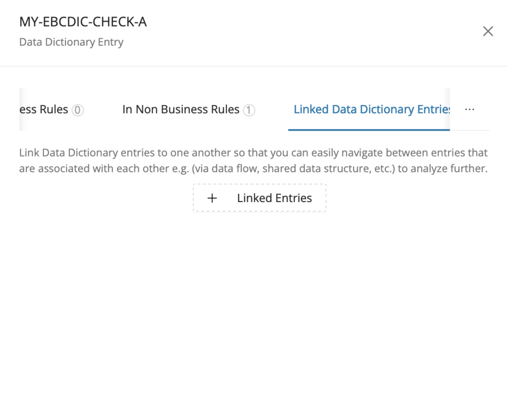
Step 4
Enter the title of the group of linked entries, provide an optional description, and click in the Link New DD Entries field to select fields to link and click Add .
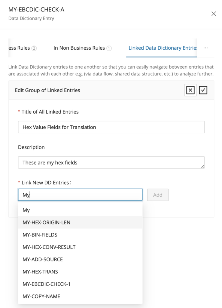
Step 5
Click the button and click Save to complete the Data Dictionary entry linking.
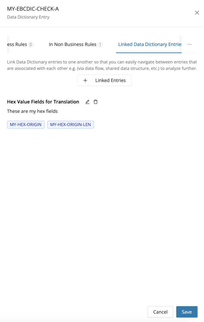
Editing a group of linked entries
Click the edit icon to enable the editing of a group of linked DD entries.
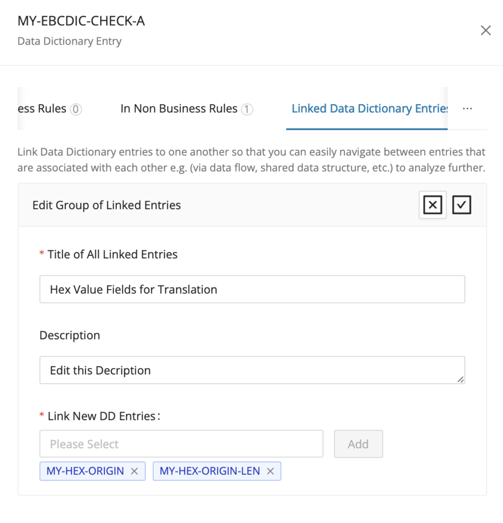
Deleting a group of linked entries
The delete icon is located to the right of the edit icon, enabling the removal of a group of linked DD entries.
Searching the Data Dictionary for linked entry groups
After linking Data Dictionary Entries and giving them meaningful group names, it is also possible to easily search at the group level from the Data Dictionary tables based on those group names.
Step 1
Open the Data Dictionary Reporting page and click the down arrow next to the title Data Dictionary to open the available saved searches.
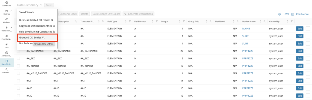
Step 2
From the list of available custom and global saved searches, select Grouped DD Entries. This shows the Group Names and Linked Data Dictionary entries in the table.
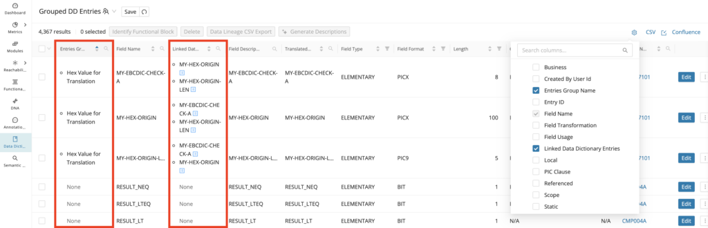
Step 3
The Entries Group Name column is sorted alphabetically, A-Z by default, and you can click the search icon to search for a specific group name if you know in advance (includes wildcard usage). Additionally, you open the Data Dictionary editor for any of the linked entries that are part of the group under the Linked Data Dictionary Entries column by clicking the blue side panel icon next to each entry in the list.
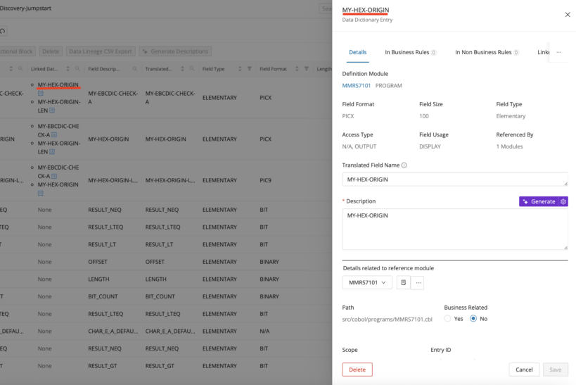
Business Variables
Business variables are fields that are identified to have some business relevance within the project codebase. These variables are either used as the target result field for a computation/transformation statement or are used in input-output operations transferring data between the program and an external data source, for example, (Resource File, Database Table, etc.), which raises a high level of confidence that the data they hold is relevant to business purposes. For COBOL, these are the variables used to extract the underlying annotated business rules. Both business variables and annotated business rules are identified when executing Identify Candidates from the Modules Reporting page.
Viewing Business Variables in Mining
To display the identified Business Variables on your project, open the Data Dictionary Reporting page and click the down arrow next to the title Data Dictionary to open the available saved searches. From the drop-down list, select Business Related DD Entries.
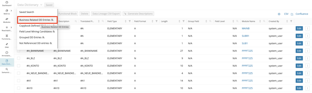
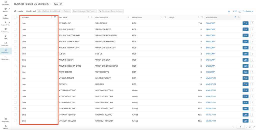
Alternatively, you can click the settings icon in the top right corner and select Base Data > Business:
The Data Dictionary table now contains a new column, “Business”. To display only business variables in the table, click the filter icon next to the column name “Business” and check true:
The table now displays the identified business variables.
The data dictionary entry of a module also indicates whether the data dictionary is a business variable. Click Edit . The displayed Data Dictionary entry contains a "Business Related" field with "Yes" set as default.
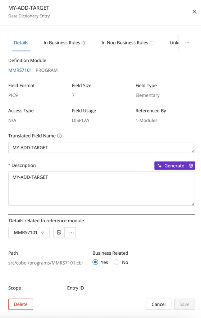
Data Dictionary attributes
In the Data Dictionary Editor inside the mining UI, you can see a few readable and editable data dictionary attribute fields. These attributes combine system-derived metadata with fields that users can maintain manually. The sections below distinguish which values are read-only and which ones can be edited during curation.
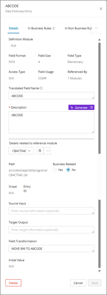
Read only Data Dictionary attribute fields:
-
Definition Module: the module where the data dictionary entry field is defined.
-
Field Name (top-left corner): the name of the data dictionary entry field.
-
Field Format: the data dictionary entry field format, for example, (PIC9, PICX).
-
Referenced By: indicates the total number of modules that reference the Data Dictionary Entry field.
-
Field Size: data Dictionary entry field size.
-
Access Type: indicates how the field is accessed with the codebase, for example, (Write, Read, UI Input/Output, etc.).
-
Scope: the identified scope or usage of the data dictionary entry field, for example, (Calls, CICS UI, Database I/O, etc.).
-
Field Type: indicates whether the field is declared at the parent GROUP level or if it is an ELEMENTARY level defined field.
-
Field Usage: shows the internal of the USAGE clause for COBOL fields, for example, (COMP, DISPLAY, etc.).
-
Path: shows the file path to the module that defines the field.
-
Initial Value: shows the literal value that the field is initialized with.
Edit-based Data Dictionary attribute fields:
-
Description: the description of the data dictionary entry field.
-
Translated Field Name: used as an alternate name for the field with greater meaning. Used in the English Translation of referencing annotations.
-
Business Related: indicates whether the data dictionary field is business-related with yes/no radio buttons, which is a single select.
-
Field Transformation: line of code where the data dictionary entry field's final value is computed or a value is moved into it
-
Source Input: any manually defined source/input information about the data dictionary entry field.
-
Target Output: any manually defined target/output information about the data dictionary entry field.
All of these view and edit-based data fields will be visible while creating new data dictionary entries or while editing existing data dictionary entries.
Java-related Data Dictionary attribute fields
-
Access Modifier: (Private, Public, Protected)
-
Local: (True, False) Class-level vs Locally Defined Variable
-
Static: (True, False) Per Instance vs Per Class Variable
Non-business related Data Dictionary entries
Users can manually change the Data Dictionary entry to Non-Business related.
Step 1:
Click Edit from the Data Dictionary page for an entry that is Business Related.

Step 2:
Select No in the Business Related field.
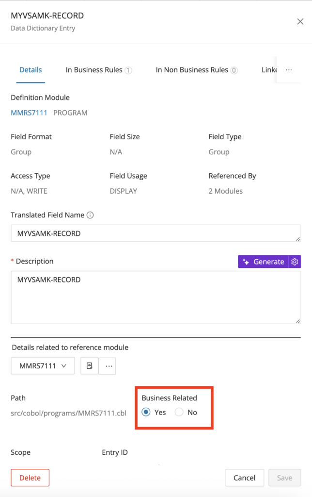
Step 3:
After clicking Save , a confirmation window appears displaying the annotation(s) that contain the reference to this data dictionary with the option to either Skip or Review.
Step 4:
Click Review to verify the annotation(s) and go to the Annotations page displaying the referenced annotation. Alternatively, if no verification is required, click Skip .
Data Lineage
You can launch Data Lineage from a Data Dictionary entry to trace how a field moves through the application. This is useful when you begin from a data element rather than from source code. Follow the Data Lineage page for the full workflow and graph options.
Annotation referencing entry
The Data Dictionary not only provides metadata about the different data entries of your project, but it also shows at a glance all of the annotated code that references each entry, as data and code go hand in hand to provide greater context on your codebase. For Data Dictionary entries, all of the associated annotated Type Rule annotations are linked for quick reference from the Data Dictionary tables (viewing all entries) or the Data Dictionary editor (viewing a single entry).
Viewing referenced Annotations
To display the column “Annotation Referencing Entry”, click the settings icon in the top right corner and select Base Data > Annotation Referencing Entry.
The column contains a list of annotations and links to each annotation candidate of type "RULE" after executing Identify Candidates.
From the Data Dictionary tables
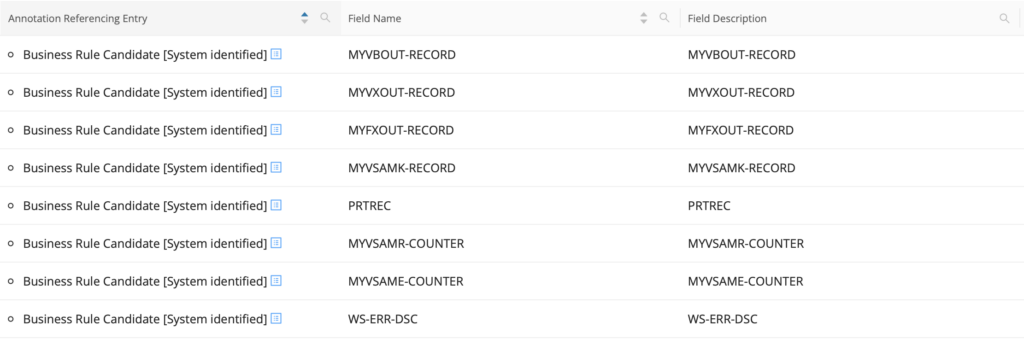
The column "Annotation Referencing Entry" only contains entries if the Data Dictionary entry is referenced by any annotations of Type Rule. Clicking the blue side panel icon next to the annotation description opens the associated annotation in the Data Dictionary editor.
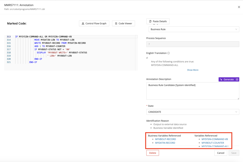
The Annotation drawer contains the section "Business Variables Referenced" and "Variables Referenced" with a list of referenced Data Dictionary entries for this specific annotation. This link is bi-directional, so that clicking the hyperlinked entries in these sections opens the associated Data Dictionary Editor per entry.
From the Data Dictionary editor
Open the Data Dictionary Editor from the Data Dictionary table or from the CodeViewer and scroll right from the "Details" tab to either the "In Business Rules" or "In Non Business Rules" tabs. From here, you can click the edit icon to make edits to the referencing annotations or click the delete icon to delete the referencing annotations.
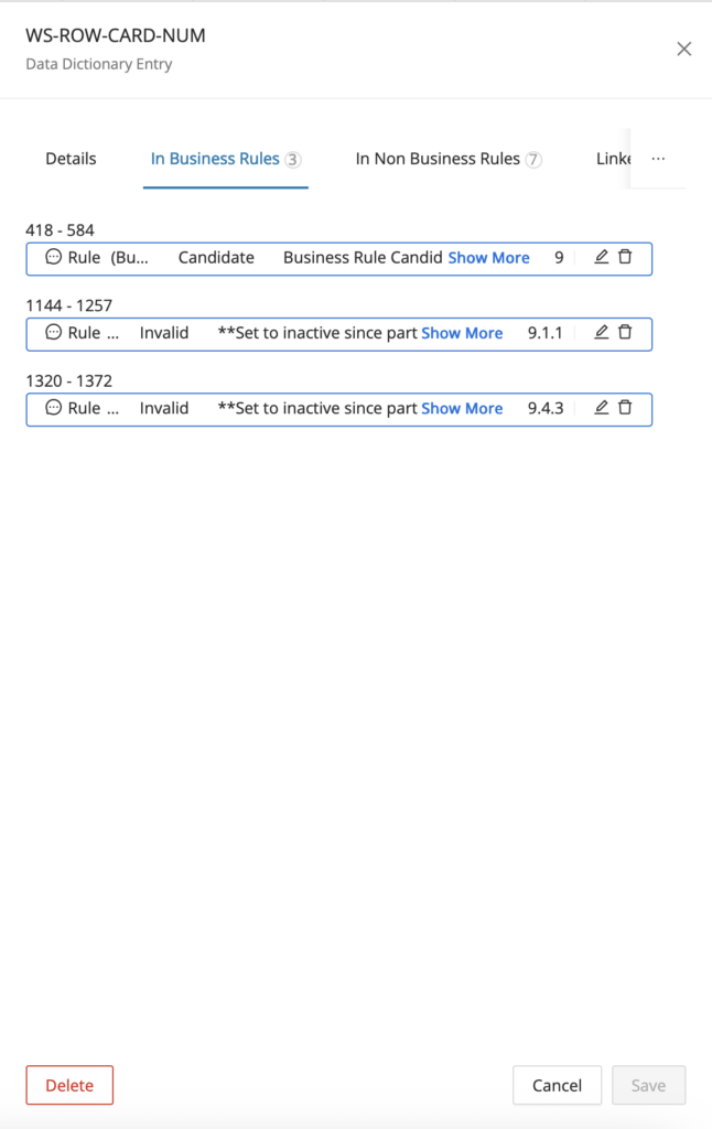
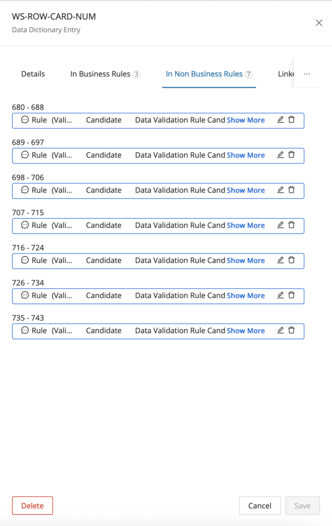
Identify Functional Block
You can also trigger Functional Analysis from supported Data Dictionary entries. This lets you move from a field-centric investigation into the related functional behavior captured across modules. Follow the Functional Analysis page for Field Level Mining for the full workflow.
Bulk entry deletion
Rather than open the Data Dictionary Editor for every entry you would like to remove from the Data Dictionary, you can do bulk deletion directly from the Data Dictionary reporting page by searching or filtering for the entries you would like to remove and selecting them in the table before clicking the delete button in the toolbar. Use this workflow when saved searches or filters have already isolated the entries that are no longer needed. It helps you clean up the repository without repeating the same deletion steps one record at a time.
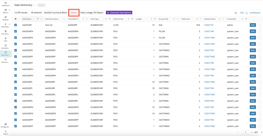
Data Lineage CSV Export
Mining provides automation via the Data Dictionary to conduct Data Flow Mapping using Data Lineage under the hood. For any field(s) selected on the Data Dictionary tables, you can click Data Lineage CSV Export in the toolbar to generate and download an Excel file showing how the data is mapped from source to target destination across the codebase. The file provides the following columns:
-
Selected Field - The field that was selected from the Data Dictionary table to base the data flow mapping on.
-
Selected Field Module - The module where the selected field is declared.
-
Selected Field Module Technology - The technology of the module where the selected field is declared.
-
Selected Field Module Type - The Type of the module where the selected field is declared.
-
Direction - Signals the upstream - from (source) or downstream - to (target) direction between the selected field module and the data module.
-
Data Module - Where the data is ultimately coming from (source module) or going to (target module). This is typically an external data source, for example, (Resource File, SQL Table, etc.).
-
Data Module Technology - The technology of the module where the data is ultimately coming from or going to.
-
Data Module Type - The Type of the module where the data is ultimately coming from or going to.
-
Transformation Statements - Shows the ordered transformation statements on the data flow path.
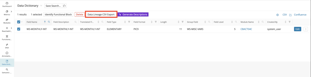
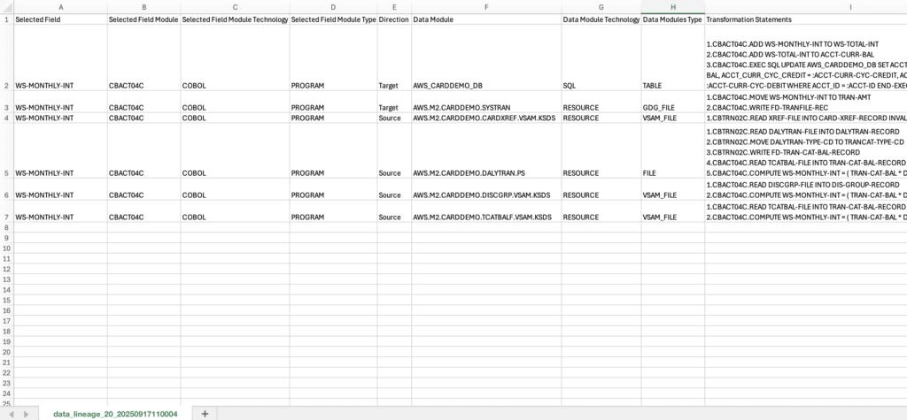
Bulk generation of Data Dictionary descriptions
Generate Descriptions is present on the Data Dictionary page, which allows users to bulk-generate Data Dictionary descriptions directly from the Data Dictionary page. This feature helps you draft descriptions consistently across multiple entries. It is most useful after discovery or candidate identification has populated a large set of fields that still need readable summaries.
Step 1:
Select two or more Data Dictionary entries and click Generate Descriptions .
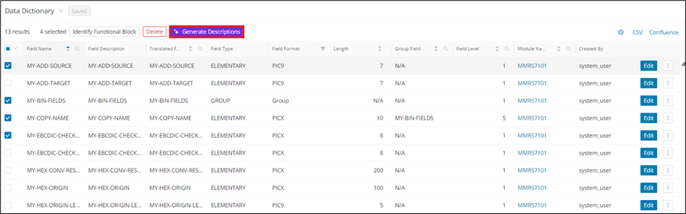
Step 2:
Click the checkbox if you want to overwrite the existing Description and click Generate .
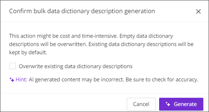
Custom properties for the Data Dictionary
Finally, you can use custom properties to expand the attributes stored for each Data Dictionary Entry. Similar to the use of custom properties across Mining, you can create custom String Input, String Repeater, URL, and Select Tag fields and edit them for each Data Dictionary Entry to provide additional context, for example, (industry or client-specific meaning surrounding the entry).
Specify the custom property while creating or editing a data dictionary entry from the Data Dictionary Editor.
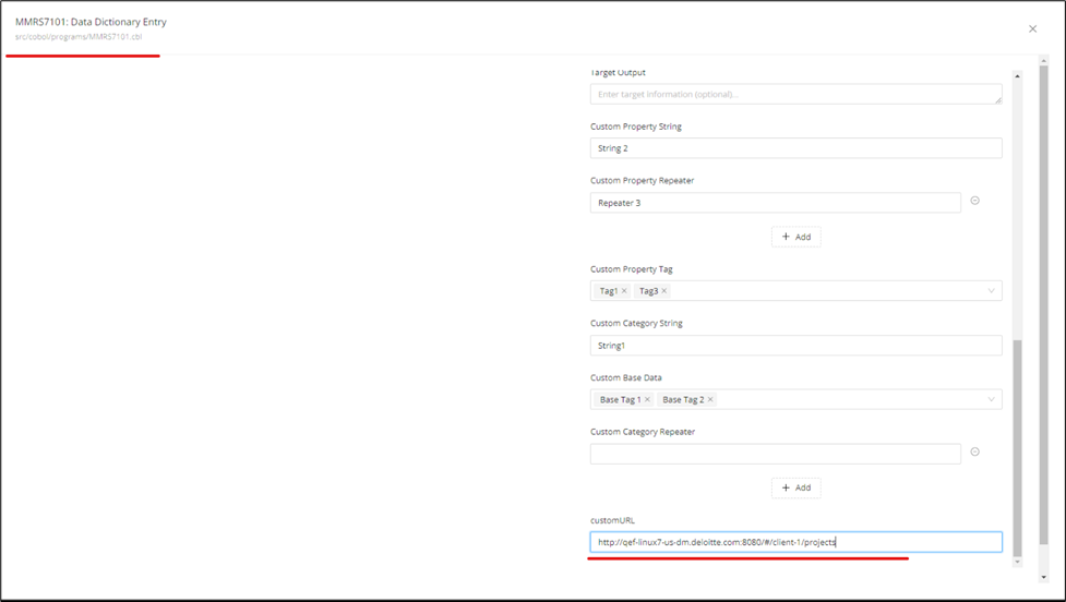
Then, from the Data Dictionary tables, you can add the custom property as a column where Data Dictionary entries can be sorted, filtered, or searched based on the custom property data.
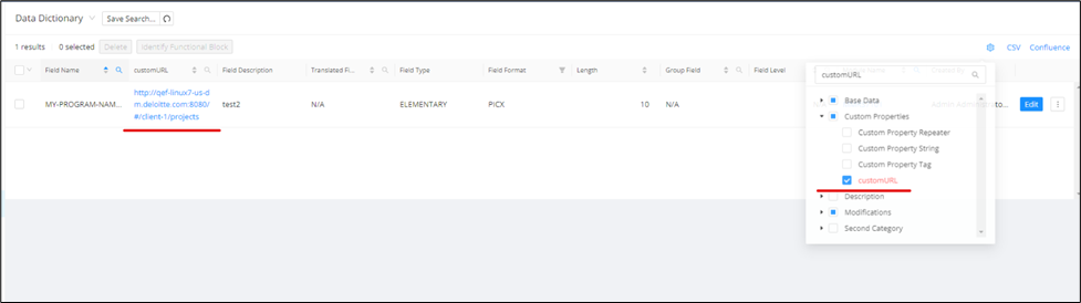
Configuration
The Configuration chapter guides you through the essential tools and settings available in the Code Discovery & Mining UI for customizing your project environment. Here, you’ll learn how to manage custom properties and imports to tailor the platform to your specific needs.
Custom properties
Each project has specific information that must be collected during mining, which could use the help of custom metadata. The following chapter describes each available custom property type and provides step-by-step instructions for managing custom properties.
Info
Custom properties are supported for Annotations, Data Dictionary, Modules, and Functional Blocks.
The following custom property types can be created:
-
Input String
-
String Repeater
-
Select Tag
-
URL
The following table lists examples of supported types, their UI representation, and corresponding example queries.
Type
Description
Input String

The Input String type is rendered in the UI as a simple text field, allowing input of a single-line text value.
String Repeater
The String Repeater type is rendered in the UI as an expandable list of text fields, allowing input of a single-line text value in each field.
Select Tag
The Select Tag type is rendered in the UI as a drop-down field, allowing:
-
selection of previously configured default tags
-
selection of existing tags created by miners
-
creation of new tags
URL
The URL type is rendered in the UI as a simple text field, allowing input of the desired URL.
Users can add or select categories for custom properties to group them in the desired category instead of using the default "Custom Properties" category.
The custom properties are visible under the defined categories in the tree view of the customizable table in the selection column.
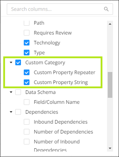
Adding custom properties
To add a custom property, navigate to the Configuration page and the desired entity tab in the Web UI.
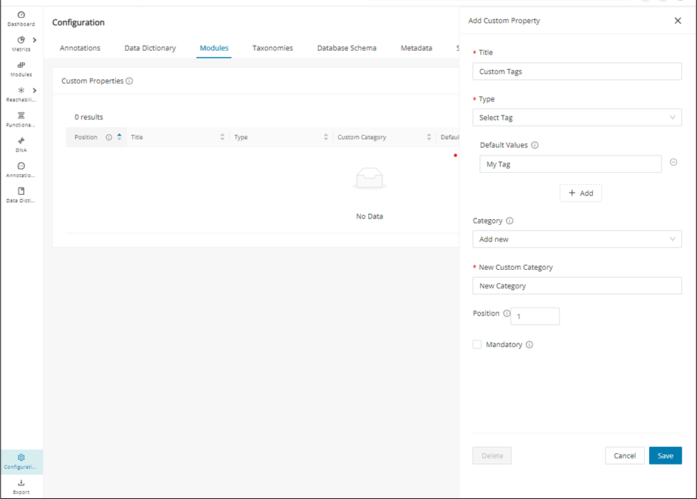
Step 1:
Click + Add in the top right corner of the custom properties table.
Step 2:
Select the title, type, category, and position of your desired property field.
If you select:
-
Select Tag as Type, add default values as needed
-
"other" as Category, add "New Custom Category"
Step 3:
Click Save to persist your changes. Your custom property will now be listed in the overview table.
Editing custom properties
Similar to property creation, custom properties can be edited in the Web UI's Configuration page.
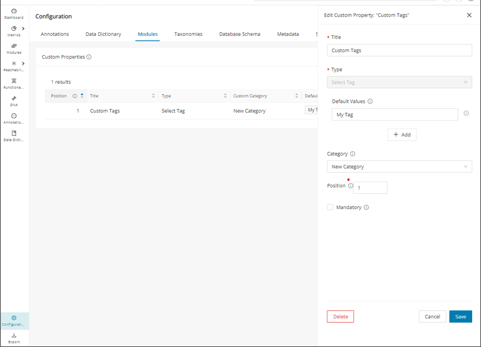
Step 1:
Click the edit icon on the right side of the custom properties table.
Step 2:
Edit the title, category, position, and default values of your property field as desired.
If you select "other" as Category, add “New Custom Category”.
Info
Note that the type of a property cannot be modified.
Step 3:
Click Save to persist your changes. Your changes are now reflected in the overview table.
Deleting custom properties
Similar to property editing, custom properties can be deleted in the Web UI's Configuration page.
Step 1:
Click the edit icon on the right side of the custom properties table.
Step 2:
Click Delete in the bottom left corner of the edit dialog, and confirm the deletion when prompted.
Searching & filtering custom properties
Once Custom Properties are configured and populated for the different supported Mining features, such as Annotations, Data Dictionary, Functional Blocks, and Modules, they can be searched and filtered just like other built-in metadata associated with those features.
Step 1
From the Annotations, Modules, or Data Dictionary tables, click the settings icon on the right next to the CSV link.
Step 2
In the settings menu, scroll down to the Custom Properties section and select your custom property(s) of interest.
Step 3
Once your custom properties are added to the customizable table, you can sort, search, or filter them (depending on the type of custom property) to find annotations, data dictionary entries, or modules that contain certain custom property values. Below is an example from the Annotations Reporting page:
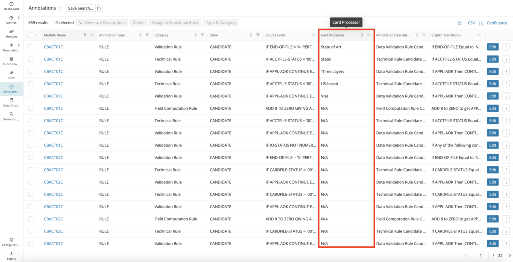
Info
Custom Properties, once added to the customizable tables, can be exported into CSV or Confluence markup same as other built-in metadata.
Annotation configuration
The Configuration page's Annotations tab allows users to create, edit, and delete annotation categories for each of the available annotation types (see Annotations).
To add a category, click + Category , enter a category name, and confirm via the tick icon next to the input field.
To edit, click the category name you would like to change to enable the input field.
To delete, select the
delete icon to the right of the category name and confirm your selection.
Configuration
Only custom categories can be edited and deleted. System default categories are not editable.
The Annotations tab also lists all available custom properties scoped to annotations, including their titles, types, default values, and the position in which they are displayed in the Annotation editor.
For information on creating, editing, and deleting custom properties, see "Custom Properties" below.
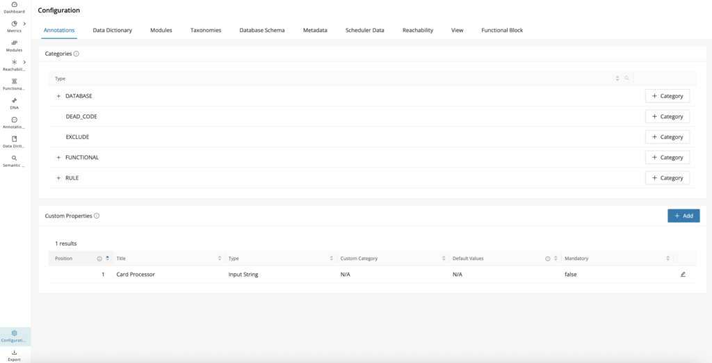
Data Dictionary configuration
The Configuration page's Data Dictionary tab lists all available custom properties scoped to the Data Dictionary, including their titles, types, default values, and the position in which they are displayed in the Data Dictionary tables and Data Dictionary editor.
For information on creating, editing, and deleting custom properties, see Custom Properties.
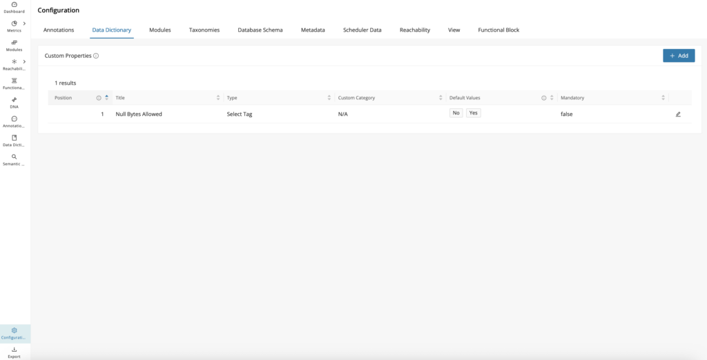
Modules configuration
The Configuration page's Modules tab lists all available custom properties scoped to Modules, including their titles, types, default values, and the position in which they are displayed in the Modules Reporting page and on the Module Details page (Custom properties Card).
For information on creating, editing, and deleting custom properties, see Custom Properties.
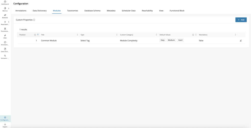
Functional Block configuration
The Configuration page's Functional Block tab lists all available custom properties scoped to Functional Blocks, including their titles, types, default values, and the position in which they are displayed in the Functional Block Creation and Editing Modals.
For information on creating, editing, and deleting custom properties, see Custom Properties.
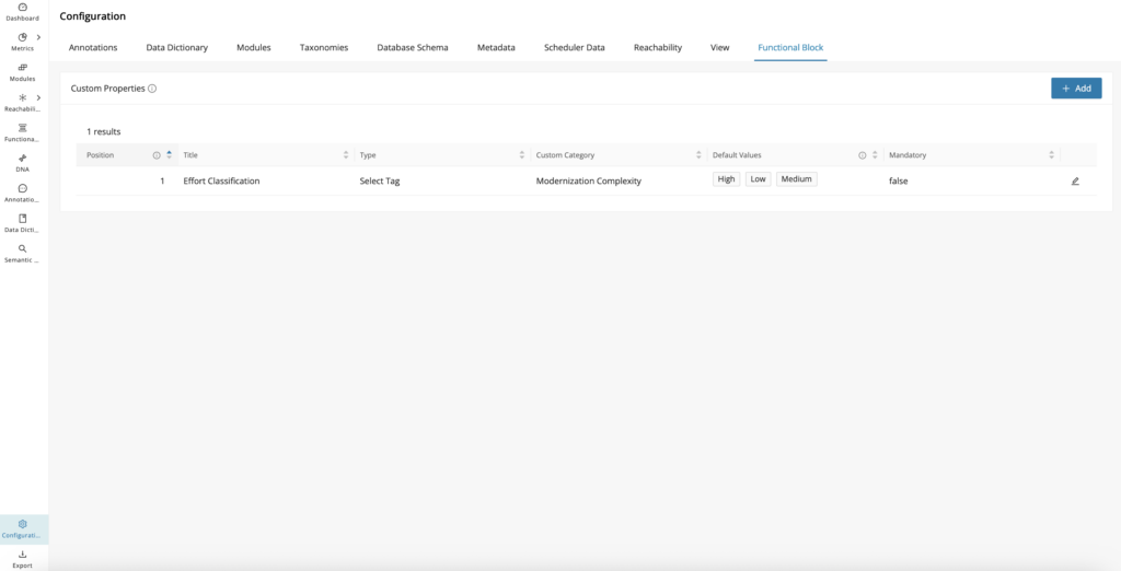
Taxonomies configuration
The Configuration page's Taxonomies tab is the main workspace for maintaining taxonomy structures in a project. It lets you review taxonomy categories, understand assignment counts, and prepare new terms before using them in analysis. The details below explain how the page reports counts and supports direct updates.
Info
This page also provides the Taxonomy Batch Import feature.
The Configuration page's Taxonomies tab lists all available taxonomies and groups them by their categories (Technical and Business Taxonomies). For each category, the number of unique modules assigned to each taxonomy is displayed.
The number of assigned modules on the right side of the Taxonomy table reflects the number of uniquely assigned modules. In the example screenshot below:
-
Categories: "Business Taxonomies" and "Technical Taxonomies"
The number reflects the number of modules with at least one business/technical taxonomy, not the number of all assigned taxonomies of each category. -
Taxonomies: "DB Access", "File Access", and "Program Type":
The number reflects the amount of modules with at least one of the taxonomy values assigned, not the sum of all values of that taxonomy, because one module can have multiple assigned taxonomy values. -
Taxonomy Terms: "Read" and "Write":
The number reflects the number of modules with the assigned term.
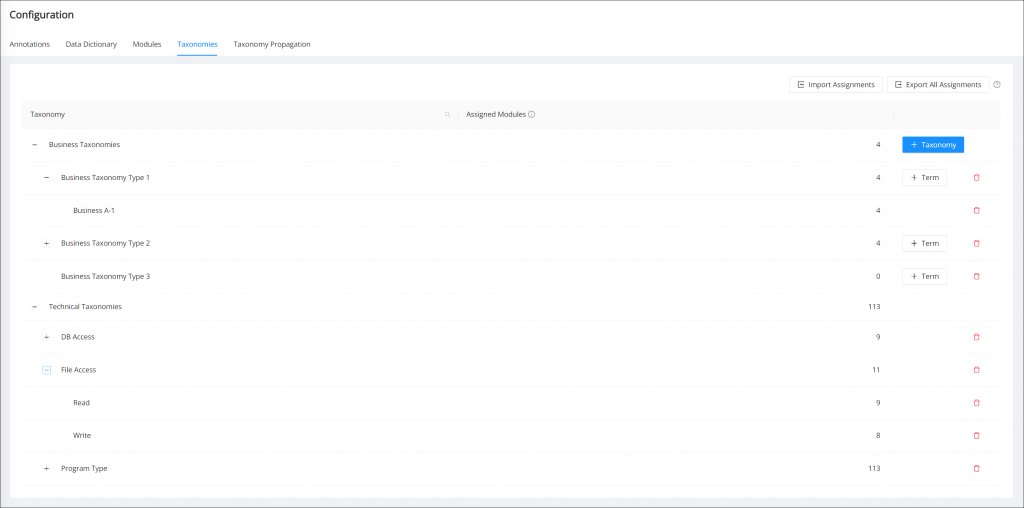
The Taxonomy column is searchable by selecting the search icon in the column header.
To add a new taxonomy to a taxonomy category, click + Taxonomy.
To add a new term to a taxonomy, click + Term.
To delete a taxonomy or term, click the delete icon for the respective row.
Info
Taxonomies and terms can be created in bulk by inserting multiple values separated by commas. In case the desired value contains a comma itself, it needs to be surrounded by double quotes.
Taxonomy batch import
Mining offers a batch import feature accompanied by a CSV template to speed up taxonomy assignments.
To get started, navigate to Configuration > Taxonomies in the Web UI and download the CSV template for your project via the Export All Assignments.
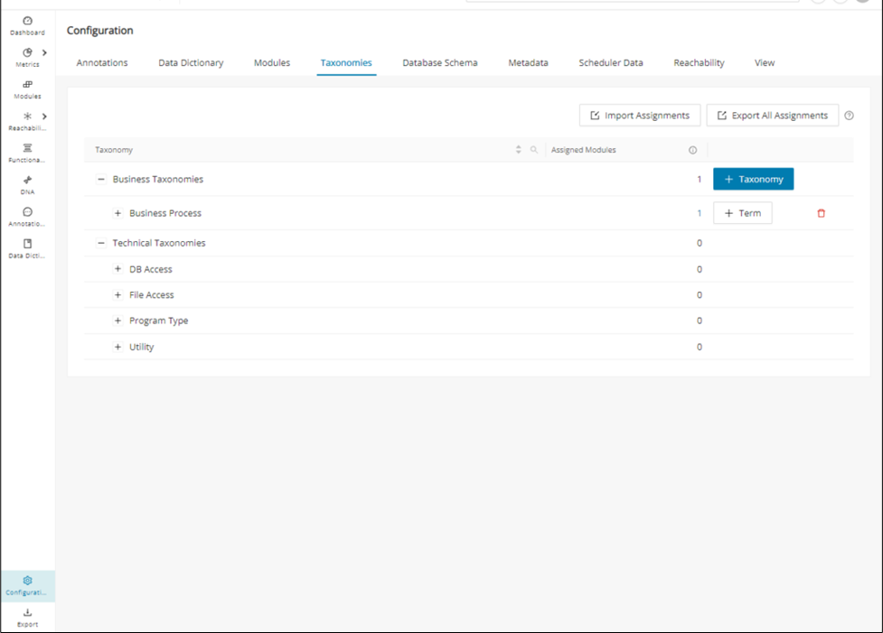
The template contains four columns used to identify a module, followed by any number of columns used to assign taxonomies. The first four columns are mandatory, and their headers must be named as follows:
| Column 1 | Column 2 | Column 3 | Column 4 |
|---|---|---|---|
| Module Name | Module Path | Technology | Type |
The remaining columns contain taxonomies (one per column) that are to be assigned to the modules.
The recommended starting point is the Export Assignments feature. Use it to download a list of the existing modules and taxonomy assignments. You can add, remove, and edit taxonomy columns in the exported template as needed.
Warning
When working with the exported CSV template, you must not modify or remove the first four columns ("Module Name", "Module Path", "Technology", "Type") to ensure that all modules can be located during the batch import. The import feature will notify you in case a module cannot be located properly.
The taxonomy import feature will only modify modules that are listed in the imported file and leave all other modules of your project untouched. This means you can remove rows, edit all or a subset of rows, or split the downloaded template into multiple parts.
This allows you to only modify the taxonomies for a part of your project, or to split the work of taxonomy assignment into smaller, independent work packages.
The following example explains how to assign Taxonomies using the template:
Our example project has 3 COBOL modules and no existing Taxonomy assignments. Downloading the taxonomy assignment using the "Export Assignments" results in a CSV file with the following content:
The file lists the modules that currently exist in the project and provides information on how to identify them. Do not alter this information.
We recommend using a CSV editor (for example, Microsoft Excel) to assign taxonomies for ease of editing in a tabular layout:
| Module Name | Module Path | Technology | Type |
|---|---|---|---|
| FIRST | src/cobol/programs/FIRST.cbl | COBOL | PROGRAM |
| SECOND | src/cobol/programs/SECOND.cbl | COBOL | PROGRAM |
| THIRD | src/cobol/programs/THIRD.cbl | COBOL | PROGRAM |
Warning
When using Excel or other CSV editors, it is imperative to ensure that one of the supported list separators is used. The taxonomy import feature requires fields in the CSV file to be separated by either comma ,, semicolon ; or tab characters. The chosen delimiter is typically auto-detected during the import step.
You can now assign taxonomies to the modules by adding new columns. For example, add a "Category" taxonomy and assign a taxonomy value to each program:
| Module Name | Module Path | Technology | Type | Category |
|---|---|---|---|---|
| FIRST | src/cobol/programs/FIRST.cbl | COBOL | PROGRAM | Security |
| SECOND | src/cobol/programs/SECOND.cbl | COBOL | PROGRAM | Utility |
| THIRD | src/cobol/programs/THIRD.cbl | COBOL | PROGRAM | Database |
When importing this file, the import will create the new "Category" Taxonomy and assign the category "Security" to the program "FIRST", the category "Utility" to the program "SECOND", and the category "Database" to the program "THIRD".
Info
Note that there are reserved Taxonomy names used by the Identify Technical Taxonomies feature, for example, File Access and Program Type. You can use and extend these Taxonomies by adding them as columns to the CSV template. When both the Identify Technical Taxonomies and Batch Import features are used, the Taxonomy assignments will be merged.
You can create more taxonomies by adding more columns. To assign multiple values for the same taxonomy to the same program, list all the values in one cell and separate the values with a comma:
| Module Name | Module Path | Technology | Type | Category | File Access |
|---|---|---|---|---|---|
| FIRST | src/cobol/programs/FIRST.cbl | COBOL | PROGRAM | Security | Read |
| SECOND | src/cobol/programs/SECOND.cbl | COBOL | PROGRAM | Utility | |
| THIRD | src/cobol/programs/THIRD.cbl | COBOL | PROGRAM | Database | Read, Write |
Here, we added another taxonomy, "File Access".
Note that the "File Access" column for the "SECOND" program is empty - the "File Access" taxonomy will not be assigned to this program.
On import, the "THIRD" program will be assigned both the "Read" and "Write" values for the "File Access" taxonomy.
To import the edited CSV file and apply the new Taxonomy assignments, use the Import Assignments on the Taxonomy overview page of the Web UI.
Info
Note that the import feature will verify the format of your CSV file and display a warning or error if the file is not compliant with the import requirements (for example, incorrect delimiters or missing columns).
Database schema configuration
Info
Uploading the SQL DDL scripts as part of your codebase project via Code Discovery will also accomplish the same goals as a DB Schema import when access to the legacy Database is not available. This includes SQL artifact module creations and Data Dictionary entry creation.
The Database Schema tab provides the capability to import database schemas to support the analysis of table structures in mining.
The imported schema information is combined with the project's discovery results to analyze and visualize inter-module data flow, variable to table mappings, and data-centric relationships and dependencies. Not only are the associated schema modules created, becoming the root module for any associated SQL tables, views, triggers, or stored procedures, but the SQL column/field information is automatically stored in the Data Dictionary.

Step 1:
A schema file in JSON format is required, which can be generated using the DB Crawler library.
Click DB Crawler to open a panel with instructions and a download option.
Step 2:
Click Download DB Crawler .
Follow the instructions to connect to your database and generate the database schema in JSON format.
Step 3:
Click Import Schema and select the JSON file.
The name of the uploaded file is now visible, followed by a table with available schema(s) that can be imported.
Step 4:
Select schemas relevant to your project from the table, then click Import selected below the table.
A success message is displayed, and the selected schemas are now shown in the Schemas in Project table
Info
A new JSON-formatted database schema file can be uploaded into Mining, which replaces previously uploaded schemas.
Step 5:
Each schema is represented by a module of language SQL and type SCHEMA.
Select one of the imported schemas by clicking the schema name to open the module details view.
This view's Contained Modules panel provides a list of objects defined in the schema.
Step 6:
Schema objects are represented by modules of language SQL and one of the following types:
SCHEMA, STORED PROCEDURE, TABLE, TRIGGER or VIEW.
Select one of the objects in the Contained Modules panel to open this object's module details view.
For example, if the selected module is of type TABLE, the tab Table Columns becomes available, displaying the respective information extracted from the database schema.
Metadata configuration
The Mining platform is a repository for knowledge about an application and its code base. The metadata tab enables you to import and export metadata. Export of metadata includes annotations, data dictionary entries, module descriptions, taxonomies, functional blocks, and custom properties in a JSON-formatted file with a timestamp.
To export the metadata, click Export metadata . To import it, click Click or drag the metadata JSON file to upload to this area .
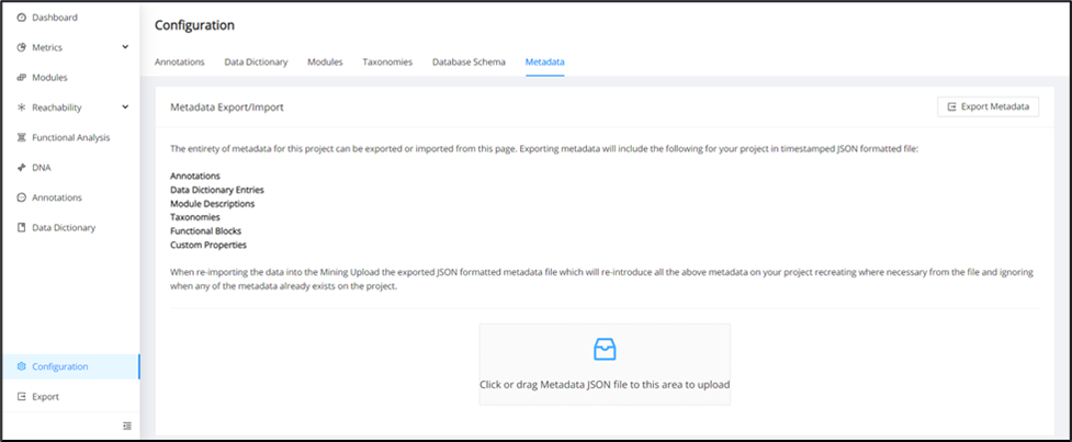
Scheduler data configuration
Control-M is a powerful workload automation software designed to streamline and automate the scheduling of various tasks and workloads. It offers a comprehensive solution for managing batch processing and other scheduled tasks across diverse IT environments. Control-M XML files containing batch scheduling and dependency information can be imported into Mining, establishing more modules and more system dependencies on those modules that could not be identified via the original Code Discovery alone. With this information available when you open the Reachability Network graph to visualize the batch system, you will be able to see any imported scheduler dependencies and how they integrate with the resource-level system.
The Scheduler Data tab is where you can import a Control-M XML file into the Mining Web UI. Click or drag the scheduler file to import.
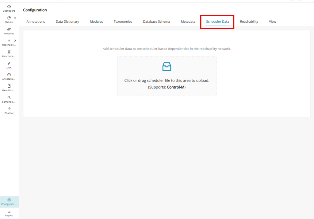
In the "Import Scheduler Data File" window, input the Identifier of the data file and click Start Import .
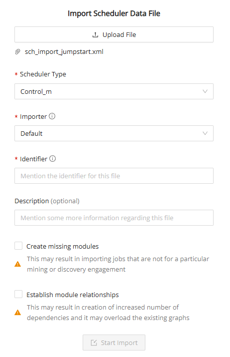
The scheduler data tab will be populated with the newly imported XML file.
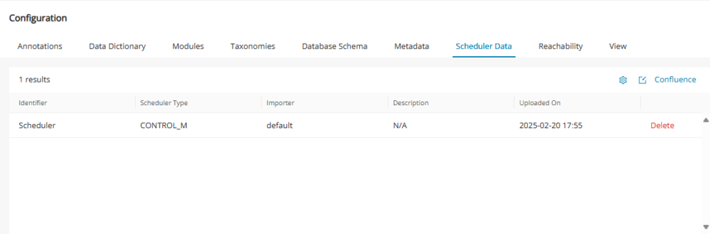
To customize the scheduler data table, click the settings icon and check the desired columns.
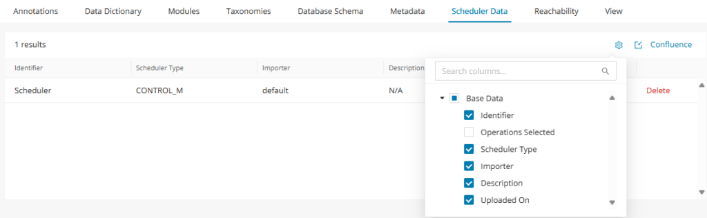
To import additional schedule data files, click the Import File icon shown below and repeat the previous steps.
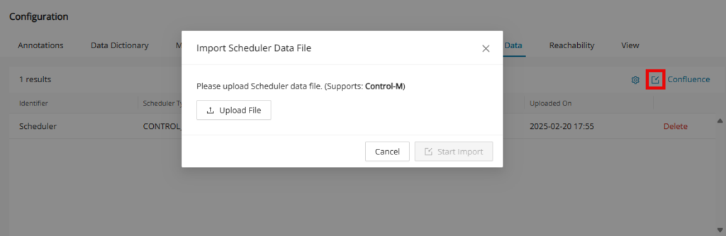
Delete scheduler import file
When a user deletes an already imported scheduler file and goes back to the reachability network, the scheduler dependencies will no longer be shown in the reachability network.
If any new module was created due to the scheduler import in the modules table, those modules will also no longer be seen in the modules table.
If call chain dependencies were previously established due to the scheduler import, they will also no longer be seen in the call chain page.
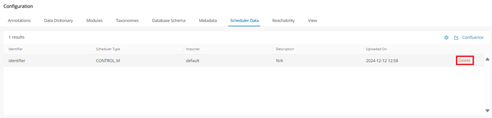
Reachability configuration
Reachability Blocks are a powerful tool for encapsulating and persisting system end-to-end flows. When generating Reachability Blocks from the Reachability Analysis page, you can configure the module technologies and types to be considered for the upper and lower bounds each time. However, if Reachability Analysis is being conducted multiple times on your project to keep consistency on which modules constitute the upper and lower bounds you can set them in the Reachability tab of the Configuration page for the entire project with no more need for ad-hoc adjustments.
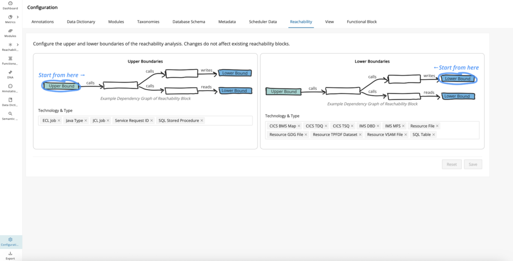
Click on the "Technology & Type" field on the left box to configure your upper bounds, and click on the same field on the right box to configure the lower bounds.
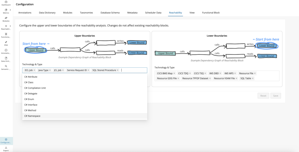
View configuration
The highlighted parser errors shown in the Mining UI are designed to signal parsing issues while ingesting a codebase project during Code Discovery. These issues could affect dependency resolutions and other downstream Mining activities, such as business rule identification and dead code calculation. However, when conducting product demos, it is not necessary to show these errors, which can distract from the overall message, so they can be disabled from the View tab on the Configuration page.
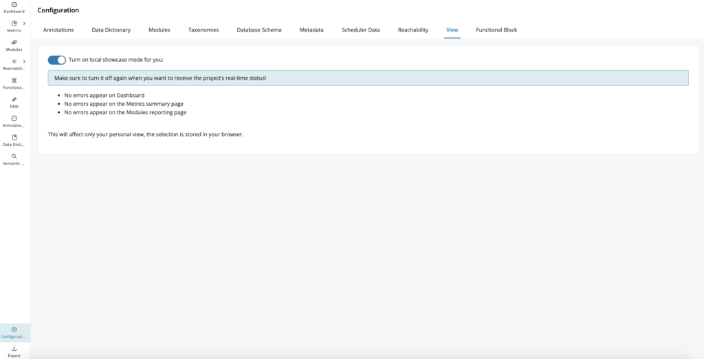

Export
All tables in the Web UI can be exported to CSV by clicking CSV in the top right corner of each table.
The Export page also allows the option of exporting the entire project data in various formats, including CSV, Excel, and GraphML.
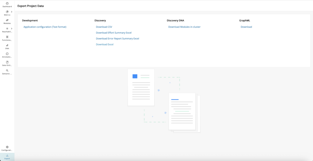
Download list
| Data Source | Download Options |
|---|---|
| Development | Application configuration (Text format) |
| Discovery |
|
| Discovery DNA | Download Modules in cluster |
| GraphML | Download business taxonomies and associated module attributes (Used for Social Graphs) |
Discovery: Download error report summary Excel
Exploring and prioritizing errors identified from Discovery is a key step in ensuring data quality and project success. To streamline this process, users can easily download a comprehensive Error Report Summary in Excel format directly from this section. Click Download Error Report Summary Excel under Discovery to download the error report summary. This provides parser errors grouped by issue type, highlighting patterns, and helps with prioritizing troubleshooting errors.
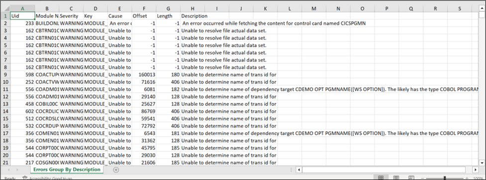
To find similar errors as a group, filter through the "Description" column.
Additional features
The Mining Web UI offers additional features that significantly enhance user experience and functionality across the entire platform. These features are meticulously integrated to ensure seamless access and usability, providing a consistent and efficient interface.
Job Framework
The Job Framework provides a list of both currently triggered and completed jobs. It gives you a central place to monitor long-running actions, review their status, and open related logs. Use it to track background processing without leaving the web UI.
To display the job list, hover your mouse over the job framework icon in the upper right corner.
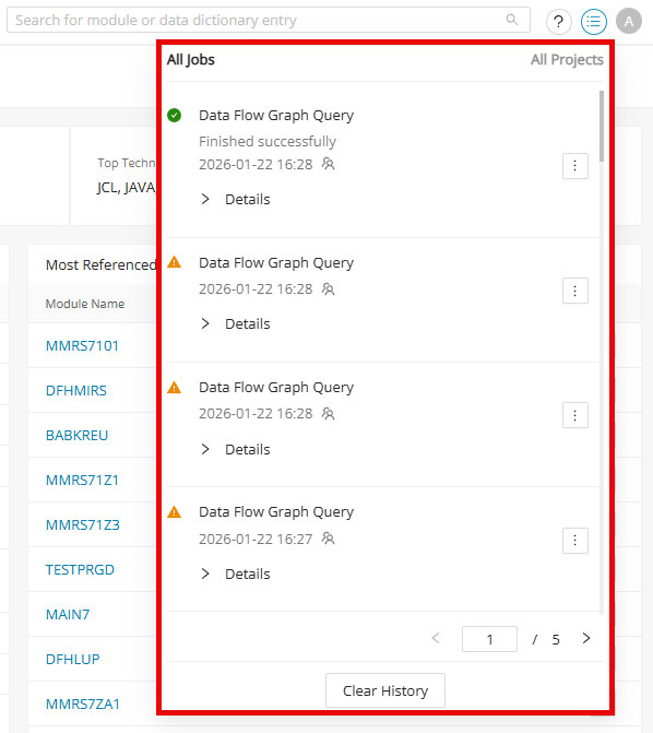
The list can contain the following information about each job:
| State | Graphical information about the job status |
|---|---|
| Running/Loading | |
| Finished Successfully | |
| Stopping/Stopped (Cancel Requested) | |
| Finished with Warning | |
| Finished with Errors | |
| Name | The name of the job. |
| Job State | Information about the status of the job as text. |
| Date and Time | Information about when the job was triggered or finished. |
| User Icon | Information via hover: who started this job (Started by) (only visible for admin users). |
| Menu Icon | Options to view the log files or remove this job from the history. When a job has the status "Running", a STOP is displayed instead of the menu icon. |
The job list displays a maximum of eight jobs per page. To display the other jobs, use the pagination element in the bottom right corner of the job list.
Show log
Each job has logged information that can be viewed by selecting Show Log from the menu icon. A dialog appears with all the logged information for that specific job. In the bottom left corner, there is a mailto link “Contact Support” to the support email.
Compare the log output with the checks in Discovery troubleshooting when a Discovery job finishes with warnings or unexpected results.
Clear history
It is possible to remove a specific job from the list or clear the entire history list.
-
To remove a specific job, select Remove from History from the menu icon next to the job.
-
To clear the entire history, click Clear History at the bottom of the job list dialog.
Users
The administrator user sees all user jobs for each project in the job list. Other users can only see their own jobs for each project. Therefore, the user icon in the job list is not displayed for them:
Notification
When a job is triggered, a notification appears with information about the running job. It contains the same information that is displayed in the job list dialog. When a job is completed, the notification contains the Show Log button, which allows you to open the log window directly from the notification. This notification disappears after a short time, but there is the additional option to close this notification manually by clicking .
Each status change of a job triggers a notification. This means that a new notification will appear when the current job gets the "Finished successfully" status.
A notification is displayed for each triggered job.
In addition to the notification, the icon in the job list changes its state and shows the same status as the triggered job. For example, if a job is currently running, the icon in the job list will display a running icon.
Show result
The following jobs will display the result after they successfully finish running.
After clicking Show Result , the jobs will redirect to the corresponding summary page as below:
-
Discovery Code completion notification redirects to the Metrics > Summary page.
-
Discovery DNA completion notification redirects to the DNA Overview page.
-
Discovery Metrics completion notification redirects to the Metrics > Summary page.
-
Taxonomy Import completion notification redirects to the Taxonomy Management UI.
-
Control Flow Graph Calculation completion notification redirects to the CFG for the module.
For example, in the "Discover DNA" job below, clicking Show Result will redirect the user to the DNA Overview page.
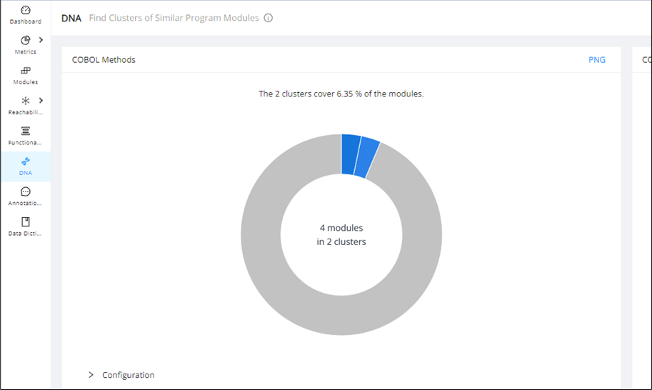
Saved Search
The Saved Search feature allows you to quickly pull up a custom table view with all of the required filters and columns. Saved Search can be found in the top left corner of the Modules, Reachability, Annotations, and Data Dictionary pages with a drop-down list that stores the default and custom saved searches.
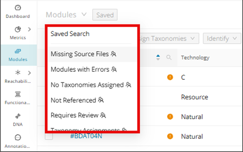
Default saved search for Modules
-
Missing Source Files
-
Modules with Errors
-
No Taxonomies Assigned
-
Not Referenced
-
Requires Review
-
Taxonomy Assignments
Default saved search for Reachability
-
Producer Reachability Blocks
-
Reachability Blocks Performing DB Operations
-
Utility Reachability Blocks
-
Reachability Blocks Performing General Operations
-
Reachability Blocks With Programs
Default saved search for Annotations
-
Business Rule Candidates
-
Database Candidates
-
Dead_Code
-
Ungrouped Annotations
Default saved search for Data Dictionary
-
Business Related DD Entries
-
Copybook Defined DD Entries
-
Field Level Mining Candidates
-
Grouped DD Entries
-
Not Referenced DD Entries
Creating and sharing Saved Search
Making any change to the default table view from the Modules, Reachability, Annotations, or Data Dictionary pages will enable the Save Search feature. For example, sorting/filtering any column (for example, Module Name) or adding a new column from the settings icon in the top right of the table view is enough to enable the Save Search... button. Click the undo icon next to the Save Search... button to return to the default table view.
When you have the desired custom table view, click Save Search... . Enter the title of the Saved Search, select the "Share With" option as required, and click Save .
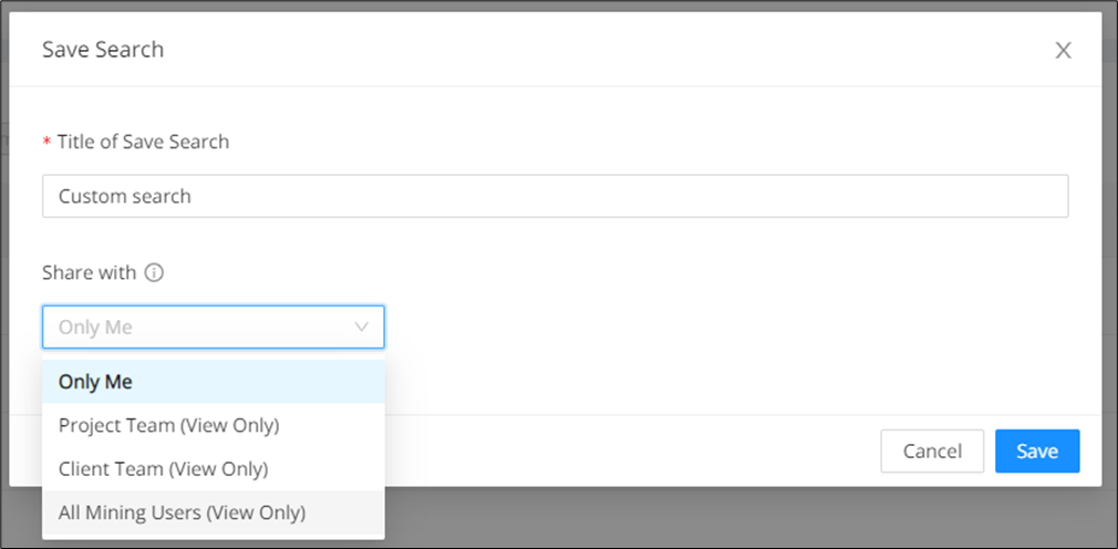
Once saved, the search created will appear in the page header drop-down list.
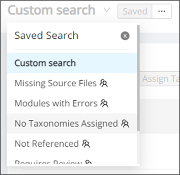
Hover over the menu next to the page header and then hover again over "Share With" to share the created search.
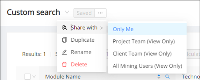
A search can be duplicated, renamed, and deleted by selecting the Duplicate, Rename, and Delete options, respectively.
Only the creator of the saved search can edit, but it can be shared with view-only access. When the saved search is shared, it can be shared with the following scope options:
-
Project Team: The search created can be viewed by all team members within the project.
-
Client Team: The search created can be viewed by all team members for all the projects with the same client.
-
All Mining Users: The search created can be viewed by all team members with administrative rights.
The team members can view the creator of the saved search. The user icon shown below is displayed next to the search name in the header, which contains a tooltip with the following information:
-
The scope of the saved search
-
The creator of the search
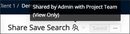
No duplicate search names are allowed on a client level. Thus, if a search is shared with the Client Team, no two projects under two different clients can have the same search name.
In the case this happens, an error message as “Duplicates not allowed” will be displayed:
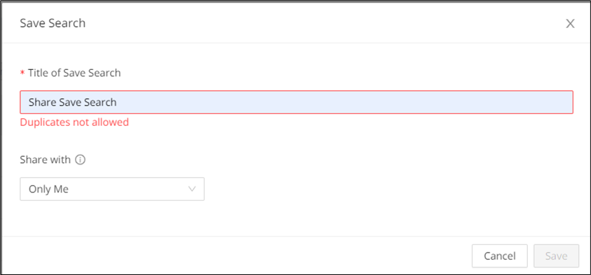
Error display
Errors and missing files will clearly and intuitively be displayed across multiple tabs, designed to streamline workflow by making it immediately obvious which items contain errors or missing files. These indicators help you spot problematic modules and views quickly while you work. Use the sections below to see where error counts and missing-file markers appear across the UI.
Error display in Dashboard
By default, the application is in real-time mode, and you can see modules with errors and missing files on the "Dashboard" page.
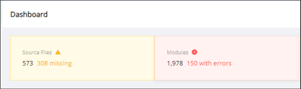
Hover over the red to read the tooltip.
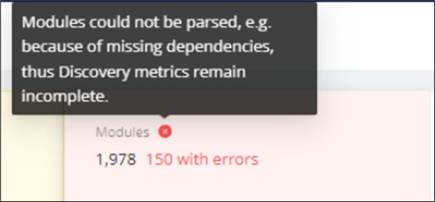
You can see the Errors column in the Metrics Summary page, which is inside the Summary table

To switch to the demo project, navigate to the Configuration page and click the View tab. Inside the view tab, switch on/off "local showcase" mode to switch to the demo project and back to the real project.
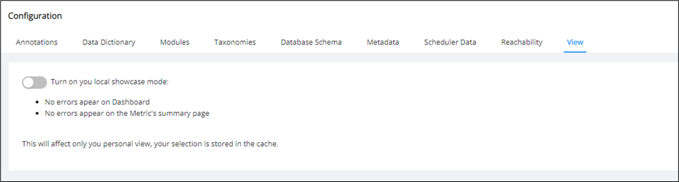
After turning on the switch, the project is switched to demo mode. The "Dashboard" page will not display the error count and icon inside the Modules section.
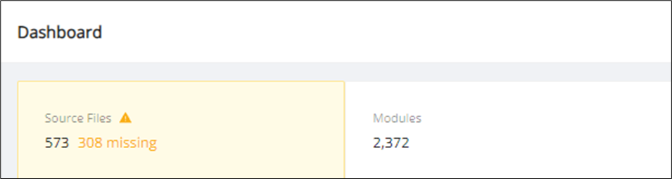
The Metrics Summary page will also no longer display the Errors column inside the summary table
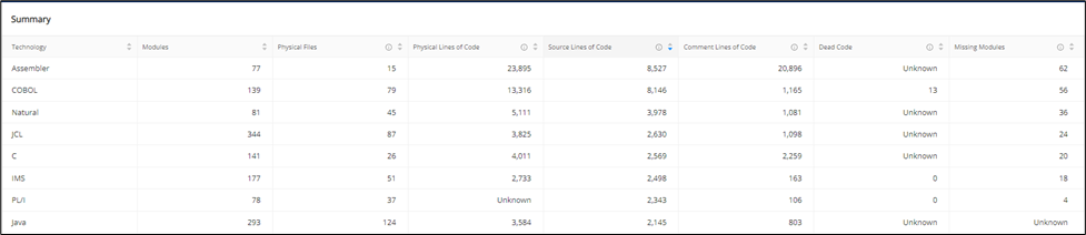
Global search for errors in Modules
Number of errors data point
In the columns list on the Modules page, the "Errors" section contains the data point "Number of errors". Check the box to add the “Number of Errors” column to the modules table.
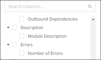
By default, the column is not filtered, but you can filter it by specifying the error count, which is a numeric value, and the filter status between =, ≤ and ≥.
When filtering the column, the entire module table is filtered out based on the applied filter.
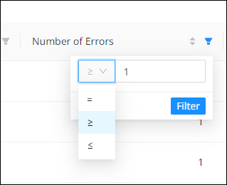
Using Global Search to find Modules with errors
On the Modules page, the global search dropdown contains the option "Modules with Errors".
If you click this option, the module table will be automatically filtered by adding by adding the column "Number of errors" to the table and setting the number of errors to "1" and the filter status to "≥".
On the Dashboard page, the clickable Modules card displays the number of modules with errors.
If you click the Modules card, you will be redirected to the Modules page with the global search "Modules with Errors".
The Results displayed in "Modules with Errors" show the same number of modules with errors as the Modules card.

Missing Modules and errors in Modules page
Missing modules or modules containing errors will have an indication next to the module's name.
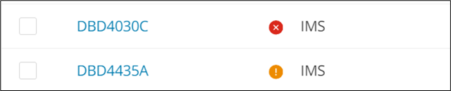
To find more specific information on the errors and warnings of a given module, click the module and switch over to the "Errors" tab.
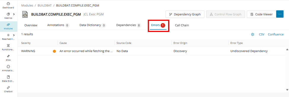
To disable this indicator, enable "local showcase mode", which can be found in the Configuration page under the View tab.
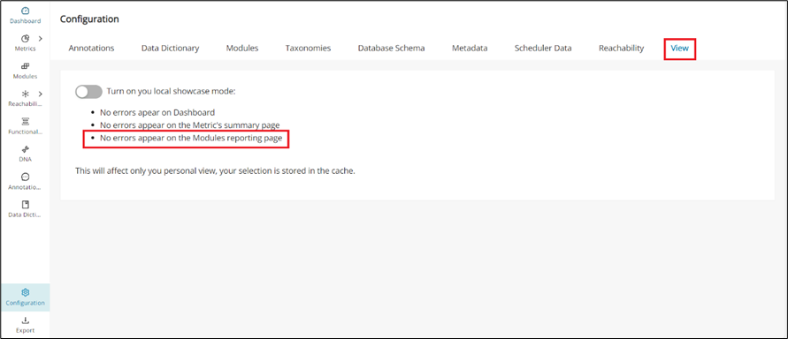
Error display in Module Details
Dependency errors on the Call Chain
In the Central Call chain page, click Render Graph and a graph will be generated.
If you have any dependency errors in the modules, the Errors/Missing Dependencies label and total count will be visible next to the Call Chain Page header.

When you click the Errors label, a new Modules table will open with the default column “Number of Errors”. The total results in this new table are equal to the number of dependency errors in the module.
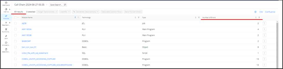
When you click the Missing Dependencies label, a new Modules table will open with the default column "Missing Dependencies". The total results in this new table are equal to the number of missing dependencies in the module.
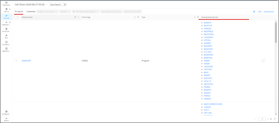
Error display in Reachability Analysis
After a Code Discovery and Reachability Analysis calculation, the dependencies that could not be properly resolved will come with an error and/or missing dependencies indicator to let you know where there were issues with the Discovery. You can find these indicators within the Reachability Analysis page from the following:
1. Block screen
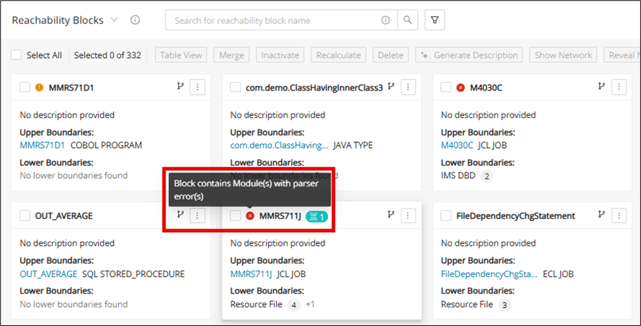
2. Block details
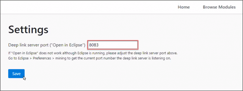
3. Table view
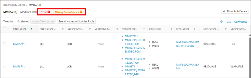
4. Graph view
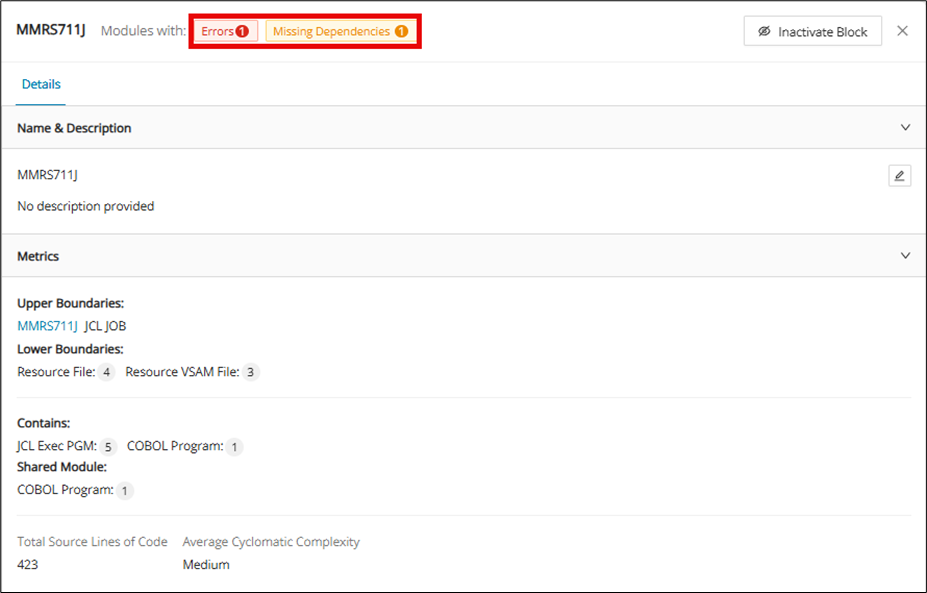
Clicking these indicators produces a new tab with a table to show the modules that have an error or missing dependency.

If a Reachability Block contained inside a Merged RB contains any errors and/or missing dependencies, the merged block will also reflect the same in the tiles view, like a single reachability block.
Table view
Tables are useful for sorting, filtering, selecting, and performing many other actions to manipulate data so that it is easier to handle. This section will detail some of the actions that the Table View in Mining Web UI has to offer.
Bulk actions
Inside the module table, the user can select a bulk number of modules by hovering over the module selection drop-down menu located just to the left of the “Module Name” column. The user can choose between two options: "Select All" to choose all the modules in the table, or "Select Current Page" to select all modules present in the current page.
If you choose "Select All" from the drop-down list, the "Deselect All" and "Deselect Current Page" options will appear in the drop-down list.
If you choose "Deselect Current Page", all modules on the current page will be deselected, and the options will be refreshed based on the status.
Now the "Select All and "Select Current Page" options appear in the drop-down menu. If you choose "Select Current Page", all modules on the current page will be selected again.
Subsequently, the "Deselect All" and "Deselect Current Page" options are displayed. If you choose "Deselect All", all modules will be deselected.
You can also press the module selection button itself to select or deselect all modules.

Filters in table view
Filter is a common feature for the table views in the Mining Web UI and is used to enable/disable which columns are shown on the table view. Simply click the settings icon, which is located at the top right of the table view, to find a drop-down of all of the available columns. To quickly find the column within the filter, type in the column name in the search bar located at the top of the filter.
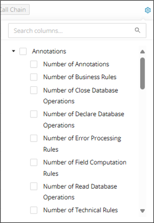
Each column has a combination of a search, sort, and/or filter function based on its specific use.
| Icon | Description |
|---|---|
Search icon, commonly used for "name" columns. Search bars with the info tooltip support wildcard search syntax abc* : search ends with "abc" *def* : search contains "def" anywhere xyz* : search starts with "xyz" |
|
|
|
Sort icon, used to sort items in this column (A-Z, Z-A, numerically). |
Category Filter icon, used to include or exclude items found within this column.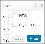 |
|
The Number Filter icon can filter numbers with the added function of =, ≥ or ≤ |
Filters in Modules page
The default columns that can be found on the Modules page are in the following order:
-
Module Name
-
Technology
-
Type
-
State
-
Last Scan
This can, of course, be customized by going into the Filter, which contains the following columns
| Category | Column | Function(s) | Additional Info |
|---|---|---|---|
| Annotations | Number of Annotations | Sort, Number Filter | |
| Number of Business Rules | Sort, Number Filter | ||
| Number of Close Database Operations | Sort, Number Filter | ||
| Number of Declare Database Operations | Sort, Number Filter | ||
| Number of Error Processing Rules | Sort, Number Filter | ||
| Number of Field Computation Rules | Sort, Number Filter | ||
| Number of Read Database Operations | Sort, Number Filter | ||
| Number of Technical Rules | Sort, Number Filter | ||
| Number of Validation Rules | Sort, Number Filter | ||
| Number of Write Database Operations | Sort, Number Filter | ||
| Percentage of Annotated Statements | Sort, Number Filter | ||
| Base Data | File Identified / File Missing | Category Filter | |
| In Codebase | Sort, Category Filter | ||
| Module Id | |||
| Module Name (Mandatory) | Sort, Search | ||
| Path | Sort, Search | ||
| Requires Review | Sort, Category Filter | ||
| Tracked Module Definement | Category Filter | ||
| Technology (Mandatory) | Sort, Category Filter | ||
| Type (Mandatory) | Sort, Category Filter | ||
| State | Sort, Category Filter | ||
| Dependencies | Inbound Dependencies | Search | |
| Missing Dependencies | Search | ||
| Number of Dependencies | Sort, Number Filter | ||
| Number of Inbound Dependencies | Sort, Number Filter | ||
| Number of Outbound Dependencies | Sort, Number Filter | ||
| Outbound Dependencies | Search | ||
| Description | Module Description | Sort, Search | |
| Errors | Number of Errors | Sort, Number Filter | |
| Metrics | Comment Lines of Code | Sort, Number Filter | |
| Complexity Level | Sort, Category Filter | ||
| Lines of Dead Code | Sort, Number Filter | ||
| Physical Lines of Code | Sort, Number Filter | ||
| Program Complexity | Sort, Number Filter | ||
| Source Lines of Code | Sort, Number Filter | ||
| Modifications | Last Modified | Sort | |
| Last Scan | Sort | ||
| Reachability Blocks | Reachability Block Name | Sort, Search | |
| Taxonomies | Number of Assigned Taxonomies | Number Filter | |
| Technical Taxonomies | DB Access | Category Filter | |
| File Access | Category Filter | ||
| Operations | Category Filter | ||
| Program Type | Category Filter | ||
| Utility | Category Filter |
Export table as CSV
Tables in the Mining Web UI can easily be exported as a .csv file by clicking CSV on the top right of the table view. Use the Filter feature to include/exclude all of the relevant columns before exporting the CSV.
For example, you can include all columns related to "Technical Taxonomies" in the table, which will then be included in the CSV export.
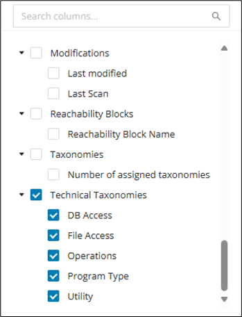
Click CSV to download the CSV file.
Export table for Confluence
Tables in the Mining Web UI can easily be exported as a .txt file, which can be used to create a table in Confluence. Use the Filter feature to include/exclude all of the relevant columns to prepare the table for export, and then click Confluence at the top right of the table view. The .txt file will be ready to download when the "Data Point Confluence Table Exporter" job is complete.
REST API with Swagger
As an alternative to the plug-in, developers can implement their own Java project to implement further functionalities using the REST API (for example, custom reports). The Swagger UI provides a browsable entry point for exploring available endpoints and request models. Use it when you want to inspect the API surface or prototype calls outside the Eclipse plug-in.
To access the REST API, open http://
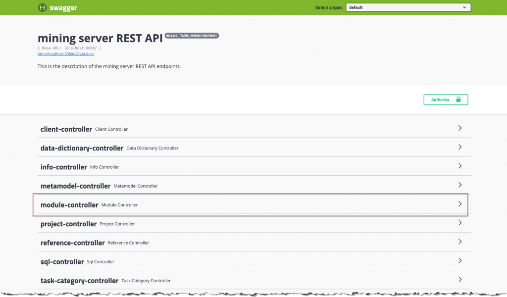
Mining Extensions
Mining Extensions are Java classes that implement a certain interface and register some additional functionality for the mining product. The extensions are registered automatically at runtime if they are put on the classpath of the mining-api-server (and they are located in the correct package).
We currently provide extension points to:
-
export mining data to a custom format
-
add additional custom pages to the Mining UI
-
provide additional MetricsContributor for Discover metrics process
Target audience
Target audience is Mining and Adoption Pod DevOps team members, as well as mining power-users and delivery professionals. These readers typically configure, extend, or operationalize Mining beyond standard end-user workflows. The remaining sections assume familiarity with Java projects, server configuration, and Mining deployment concepts.
Implementing Mining Extensions
To implement a mining extension, it is recommended to create a new Java project. Any simple Maven project that compiles to a jar file will do.
Configuring projects
You need to add the "mining-shared" dependency:
To access mining data within your application (for example, to implement an export extension), you will also want to include the "mining-data" dependency:
Warning
Disclaimer: There is currently no stable, public API available to access mining data. Therefore, include and use the "minig-data" project with the expectation that your project may break with a future update. A stable, approved API may come in the future.
Loading extensions
To load your extension into the mining-api-server, you need to compile your extension to a jar file and then add the jar file (and all of its dependencies) to the classpath of mining-api-server. All extensions that are underneath the package innowake.mining.extensions will then be automatically registered.
To add your extension to the classpath, use the loader.path system property (or the LOADER_PATH environment variable) and launch the application using the org.springframework.boot.loader.launch.PropertiesLauncher class. More information on the topic can be found here.
Example launch options from the command-line:
Use the below command for mining versions before 99.9.0-alpha-202409260030:
Info
On the command line, use the -cp option, not the -jar option to specify the mining-api-server jar file. Otherwise, the main class argument (org.springframework.boot.loader.launch.PropertiesLauncher) will be ignored.
How to ensure the extension was loaded?
Add a @PostConstruct method to your extension class in which you log the successful loading:
That way, you can check the Mining server logs to ensure that everything was set up correctly.
Showing extensions on the UI pages
You can show your extension on the export page, optionally. A "Mining Export Extension" will show itself on the export page by default, whereas a "Mining Job Extension" will not show. This option can be changed according to the requirement by overriding the method getShowOnPage() of the ShowOnPageExtension interface, inside your extension class, as shown below.
Info
Currently, Mining supports showing UI extensions only on the Export page and Customizable Tables.
It returns a ShowOnPage object, which can be created by providing values for the parameters :
-
boolean show: This accepts a boolean value.
trueif the extension should be shown on the page,falseotherwise -
String label: This accepts the string value for the label of the extension
-
String category: This accepts the string value for the category of the extension, defaults to 'Extension' if null or empty
-
String usage: This accepts the string value, which should be one of the Usage values from the Usages class if it needs to be shown in the table or 'ExportPage' to show in the export page, default to 'ExportPage' if null or empty.
- Use the following mapping for the locations
Mining Extension types
The following extensions can currently be registered – each description also includes a sample implementation. Together, they cover the main extension patterns for adding export, job, or UI-related functionality. Review the type that matches the behavior you want to introduce before starting implementation.
Mining Export Extension
Info
Eclipse Project with example implementation: mining-export-extension-example.zip.
This kind of extension contributes an export format. The export can be triggered via an HTTP request to:
Below is an example for a simple export extension:
Mining Job Extension
Info
Eclipse Project with example implementation: mining-job-extension-example.zip.
This kind of extension contributes the implementation of a Job that can be executed on a mining project and runs on the server. Unlike an export extension, a job is executed asynchronously ("in background") - its status can be observed via the Job REST API. The Job API also provides a way to cancel a Job. The Job can optionally produce a result. These feature make it the most flexible type of extension that is suitable for long-running and computationally intensive tasks.
The implementation of a Job Extension must provide a factory method that creates a Job instance. The returned instance will then be scheduled for execution via the job framework. It can be triggered via an HTTP request to:
Optional query parameters are passed in the parameters Map to the createJob() method of your extension (see below). The request body is passed as the inputDataargument and may contain arbitrary data (or it can be empty, if the job requires no input data). This allows your extension to implement file upload / import functionality.
You can implement the getParameterDescriptions() and getUploadDescription() methods to describe the parameters that can be passed to your extension, respectively, and the file that can be uploaded. This is especially useful when also overriding getShowOnExportPage() to show the extension on the Export page of the Mining UI, as it will allow users to interactively input the parameters or choose a file through the UI. Note that even when not implementing getParameterDescriptions() or getUploadDescription() it is still possible to pass parameters or upload a file when manually sending the HTTP request or using the mining-cli.
Below is an example for a simple job extension:
Mining UI Extension
Info
Eclipse Project with example implementation: mining-ui-extension-example.zip.
This kind of extension contributes a new page within the Mining UI. The page will be displayed in the navigation menu on Mining UI. It can optionally receive the id of the currently selected project and client.
When using a path as IFRAME_SRC (as in the example above) then the static resources for your extension will be served from the classpath (from one of the default locations used by Spring Boot). You can also embed an external web page in the iFrame by specifying its full URL (for example. "http://my-other-domain.com/my/extension").
In order to serve the resources (HTML etc.) for your extension from the classpath, you need an additional configuration. The default security configuration of mining-api-server will set the X-Frame-Options: DENY header on all resources. This will effectively prevent your extension from functioning since it is displayed in an iframe. Also, we enforce Authentication which may also cause problems for your static resources.
To fix this, add another class to your extension project:
Now you can put the resources for your extension under "src/main/resources/static/my/extension-url" (or whatever path you configured as IFRAME_SRC).
Please see the attached Eclipse project for a working example.
Discovery Contributor
This extension enables you to provide custom contributors for Discovery. These contributors allow you to discover new types of Modules from source code, or to extend the already supported Modules with additional information. This will be helpful for clients who have different language dialects or need to support any client specific implementation.
Info
The class implementing DiscoveryContributor or DiscoveryContributorFromSource has to be public and needs to be annotated with @Component. It also needs to be underneath the innowake.mining.extensions package.
Here is an example for an extension that extends the already discovered Java classes with additional dependency information based on a customer-specific annotation:
Metrics Contributor
This extension enables to provide custom Metrics contributors. This will be helpful for clients who have different dialects or to support any client specific implementation.
Info
The class implementing MetricsContributorExtension has to be public and needs to be annotated with @Component. It also needs to be underneath the innowake.mining.extensions package.
Technical Taxonomy identification
If a technical taxonomy has to be identified for a module based on some patterns that cannot be achieved through Taxonomy propagation (or) through the existing technical taxonomy logic, then you can write a custom logic that should implement TaxonomyIdentifier interface. Although, this interface is not introduced specifically as a mining extension, one can still use it like all other extension.
Info
The class implementing TaxonomyIdentifier<ModuleBasePojo> has to be public and needs to be annotated with @Component. It also needs to be underneath the innowake.mining.extensions package. At the time of writing, this can take AstNodePojo , AstModel , DependencyModel .
Let's say you need to identify all the Cobol modules that have a CICS statement in them as the "Access CICS" taxonomy, then:
GenAI Context Retriever
Before a prompt is sent to a GenAI model, additional context is added to the prompt by context retrievers. It is possible to add custom context retrievers with a mining extension.
To do so you need to add a class implementing one of the ContextRetriever interfaces to the innowake.mining.server.genai.context package:
-
GenAiAnnotationContextRetriever -
GenAiModuleContextRetriever -
GenAiFunctionalBlockContextRetriever -
GenAiReachabilityBlockContextRetriever -
GenAiDataDictionaryContextRetriever
It is also possible to define multiple retrievers for the same kind of entity. Each retriever is supposed to return the context of the previously executed retriever + the newly retrieved context.
Example
If you wanted to add the custom properties of an annotation to the annotation description prompt, the context retriever could look like this:
The String value that gets passed to the AiGenerationContext constructor will get added to the prompt.
Request UUID
-
If you don't use GenAI capabilities for the context retrieval you can ignore this
-
The context object (f.e.
AnnotationContext) which gets passed toretrievehas a methodgetRequestUUID -
Purpose: associate the context retrieval with the description generation for token usage tracing purposes
-
If you access f.e. the Knowledge Service in your context retriever, you should add the UUID to the request as part of the
requestMetadatamap at key "uuid"
Knowledge Cockpit
The Knowledge Cockpit is your central hub for knowledge ingestion, management, and retrieval. Here, you can leverage industry or client documentation, raw source code, or Mining metadata to build a strong knowledge repository where anyone interested in documenting or extracting information about technical systems in general and detailed terms can do so with ease. The Knowledge Cockpit integrates Mining and also the Knowledge and Prompt services to gather required information.
Categories of knowledge
There is no limit to where the documents/files the Knowledge Cockpit pulls information from originate. This means that as your core base of knowledge material grows, it becomes important to categorize it to provide the most relevant knowledge retrieval. When doing searches on available knowledge later on, you can select from the drop-down which categories of knowledge you would like the search to be based on.
Adding a category
Step 1
Click + Add Category on the top right.
Step 2
A side panel opens where you can specify the new category name and click Save .
Cloning a category
In the Categories table, select the category(s) you would like to clone and click Clone under Actions.
Deleting a category
In the Categories table, select the category(s) you would like to delete and click Delete under actions.
Merging categories
Click Merge Categories on the top right.
Renaming a category
In the Categories table, select the category(s) you would like to rename and click Rename under actions.
Ingestion of knowledge
After creating your initial categories of knowledge, you can begin to ingest documents and other files into the Knowledge service under those specific categories, making it easier to pull from the right sources later on when searching the knowledge base. There are no limits to the number of documents you can ingest, and they are uploaded via the Job Framework asynchronously so that you are free to work on other tasks in parallel.
Info
Supports PDF files, Excel files, text files, markdown files, and also source code (COBOL, Natural, PL/1, and Java).
Uploading files
Click in the middle of the UI to select files or drag your files into the UI.
Search
With the documented information and source files to extract knowledge from available you can begin to search for this information. Very generic search queries can be issued, so it does not require having in-depth personal knowledge about which documents or files certain information should be found; you can simply query and explore with only a high-level understanding of the file system. With Knowledge cockpit search, you can forgo the extensive manual analysis to find information about your system in favor of quick semantic queries such as "Where is interest calculated?" or "Where does ticket issuance occur?".
Info
For better results, select the most relevant category of knowledge before your search and adjust the prompt (via Prompt service) to tailor the depth and general understandability of the responses.
Select one or more categories of knowledge to base your search on.
Your search results can be copied to the clipboard for faster and more efficient knowledge retrieval in the future by clicking the copy icon on the top right of the results card. You can also save a memory snapshot of the search query and result by clicking the save icon.
Scrolling down past the search results, you will also see the actual documents used to produce the search results for reference.
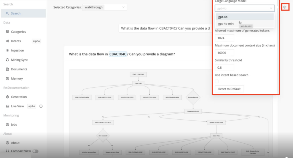
You can configure semantic search based on your desired results directly from the search page by clicking the settings icon on the far top right corner. This includes the selection of the LLM (Large Language Model) used, maximum generated token, maximum document size, and more.
Memory
You can save the results from your search as a memory snapshot in the database (under a knowledge category) for future reference when searching. When the system encounters a question that is similar to one from the memory snapshot, it can quickly refer to it. The Memory page provides a place where all of your saved memory snapshots can be managed, including seeing the query in memory and what the result was. Additionally, you can delete memory snapshots that are no longer relevant.
Mining Sync
As the Knowledge service integrates with the Mining API server, here you can select a Mining project, and you’ll have the option to sync all of the Mining project’s modules or just selected modules. The available Module and Functional Block descriptions will be ingested into the Knowledge service, scoped to your selected knowledge category, bolstering the search output around this project when using the category of knowledge. You can also reprocess modules that have already been ingested previously.
Info
This feature depends on the Mining data (Module and/or Functional Block Descriptions) already being available within the Mining project.
Select your mining project that has the modules whose descriptions you would like incorporated into the Knowledge service.
After selecting the Mining project of interest, you can select all or cherry-pick the modules you would like to sync with the Knowledge service and click Sync selected modules .
ReDocumentation
Create sophisticated documentation for COBOL modules. First, select the modules you would like to document. You can auto-tag modules here, similar to taxonomies, to describe and document their business domain along with their purpose. Once the tags are created, you can execute auto tagging, where the LLM will look at the source and decide which module is applicable to apply the tag. Alternatively, you can sync in existing taxonomies from Mining. This also requires that you do the source code (needed by redocumentation) ingestion, as the Mining sync only pulls in the descriptions.
You can view the generated documentation in Live View mode, or you can click the Download Result.zip button on the generation page to download the zipped markdown files.
Also, the generated documentation can be added as knowledge under your specified knowledge category
Info
The documented module descriptions that are generated are built from scratch using the source files and do not take into account existing module or Functional Block descriptions from Mining.
Setup
Before generating the documentation, you'll need to set up the LLMs (Large Language Models) you would like to use for code explanation, code generation, and reasoning. The Knowledge Cockpit provides flexible integration with a range of LLMs, including Azure OpenAI, Antropic Claude, and LLMs provided via AWS Bedrock.
Select your LLMs of choice and click Next .
Documentation generation
After the documentation setup stage, you are ready to begin generating documentation for selected modules. Additionally, here you conduct tag management and auto-tagging of your selected modules to classify within the documentation which application business domain each module should be classified with.
Auto-Tagging
You can either manually create tags to classify modules under business domains, or you can sync taxonomies from Mining if they already exist.
Step 1
Click Open Tag Management .
Step 2
In the Side Panel that opens, either click Sync Taxonomies to pull in taxonomies from Mining, or you can manually tag names/descriptions and click Add .
Step 3
Close the side panel and click Execute Auto-Tagging to automatically assign tags to modules.
Generate Markdown
Once your modules are autotagged, click Generate Markdown button to trigger the documentation generation job. Upon completion, you can click Download Result.Zip to download a zipped package of the documentation (markdown files), or you can view the results directly in the UI can navigating to the "Live View" page on the main menu under Re:Documentation.
Live View
Once you have generated the markdown files for the documentation, you can view this auto-generated documentation directly in the UI by clicking on Live View in the left main menu under ReDocumentation. There will be an Index page overviewing the entire application based on the selected modules and individual detail pages per module.
Index page
Summary of the purpose of the application.
Module page - Table of contents
The Table of Contents provides an overview of the documentation on each module with hyperlinks to quickly jump to each section.
Module page - Description
Summary overview of the purpose of each module.
Module page - Partitions graph
Shows how the different sections and subroutines of a program are called graphically.
Module page - Field references
Provides a summary overview of all the fields referenced inside the program, including descriptions and the potential values they may store.
Module page - Partitions
Provides a summary breakdown of each of the different sections and subroutines of a program, explaining the functional workflows while showing the associated source code.
Prompt management
The prompts contain the exact instructions provided to the AI models on how to generate a response to a particular query, including the GenAI features in Mining (Annotation Descriptions, Module Descriptions, etc.), and also Knowledge Cockpit semantic search and documentation generation. Within the prompt management page, you add new prompts or edit/delete existing prompts based on your tailored response needs.
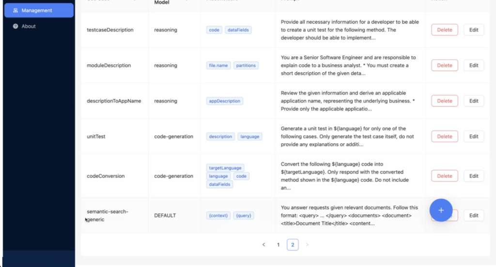
Release Notes
Imprint
Germany
Deloitte innoWake GmbH
Robert-Bosch-Str. 1, D-89250 Senden
Phone: +49.7307.92190.111
Mail: amiproductsupport@deloitte.com
United States
Deloitte LLP 30 Rockefeller Plaza, New York, NY 10112
Phone: +1.800.769.0480
Mail: amiproductsupport@deloitte.com
Deloitte refers to one or more of Deloitte Touche Tohmatsu Limited, a UK private company limited by guarantee ("DTTL"), its network of member firms, and their related entities. DTTL and each of its member firms are legally separate and independent entities. DTTL (also referred to as "Deloitte Global") does not provide services to clients. In the United States, Deloitte refers to one or more of the US member firms of DTTL, their related entities that operate using the "Deloitte" name in the United States and their respective affiliates. Certain services may not be available to attest clients under the rules and regulations of public accounting. Please see http://www.deloitte.com/about to learn more about our global network of member firms. © 2026. Deloitte. All rights reserved
© 2026. Deloitte. All rights reserved.